14 Computed Tomography
Contents
14 Computed Tomography#
14.1 Motivation and concept#
One important application of fourier transforms is x-ray Computed Tomography which, in medicine, is called a CAT scan and is used to observe soft tissue inside a person’s body. The method is quite general and can be used in diverse applications, for example, to measure the position and concentration of different chemical species in a combustion reaction (i.e. in a flame) or to examine the quality of steel inside steel-reinforced concrete. Waves, which could be electromagnetic or acoustic, are passed through an object and the absorption at many points along a line is measured and then this is repeated at each of many angles. After transforming, this data can reproduce an accurate image of the original object. Houndsfield and Cormack received the 1979 Nobel prize in Physiology or Medicine for discovering the technique of x-ray computed tomography.
The method consists of two parts, first is the acquisition of the data the second is unscrambling this to form an image. The second part is purely mathematical and reconstructs the image on a grid of points, i.e. a 2D array or matrix, which we shall call the image plane. In a CAT scan a thin sheet of x-rays passes through the object and the intensity of the radiation emerging at each point across the x-ray sheet is measured relative to its initial value. Nowadays, a multi-element detector such as a CCD device could be used. Any difference in signal amplitude is due to absorption of the x-rays, but there must not be any significant refraction or scattering caused by different densities as this will mix up different spatial positions. In the next and subsequent steps both the source and detector are rotated by a small angle and the process repeated to cover a \(180^\text{o}\) range. (In practice the source and detector spin round the patient which is why the CAT scan machine is formed as a hollow cylinder). The signal at each angle is then fourier transformed, filtered as required, and back transformed and re-assembled in clockwise fashion to form an image. To get an idea of how this happens Figures 86 and 87 show the process in schematic form.
The principle is shown in the next few figures; the necessity to rotate the source and detector to observe details is clear: at any given angle the total absorption along any ray is measured so any 2D information is integrated and only 1D information remains, see figure 86.
The extent of absorption is given by Beer’s Law, which for the simple case of a solution in a cuvette in a spectrophotometer is
where \(I_0\) is the initial intensity at \(x=0\), \(\epsilon_\lambda\) the extinction coefficient at wavelength \(\lambda\) and is a characteristic of the molecule and describes how strongly the molecule absorbs, the concentration is \([C]\) and integration is over path length from \(x=0\to l\). We shall assume that the x-rays used in CAT scans are collimated, i.e. made up of pencil like rays, and sufficiently monochromatic that the absorption is equal across its spread of wavelengths.
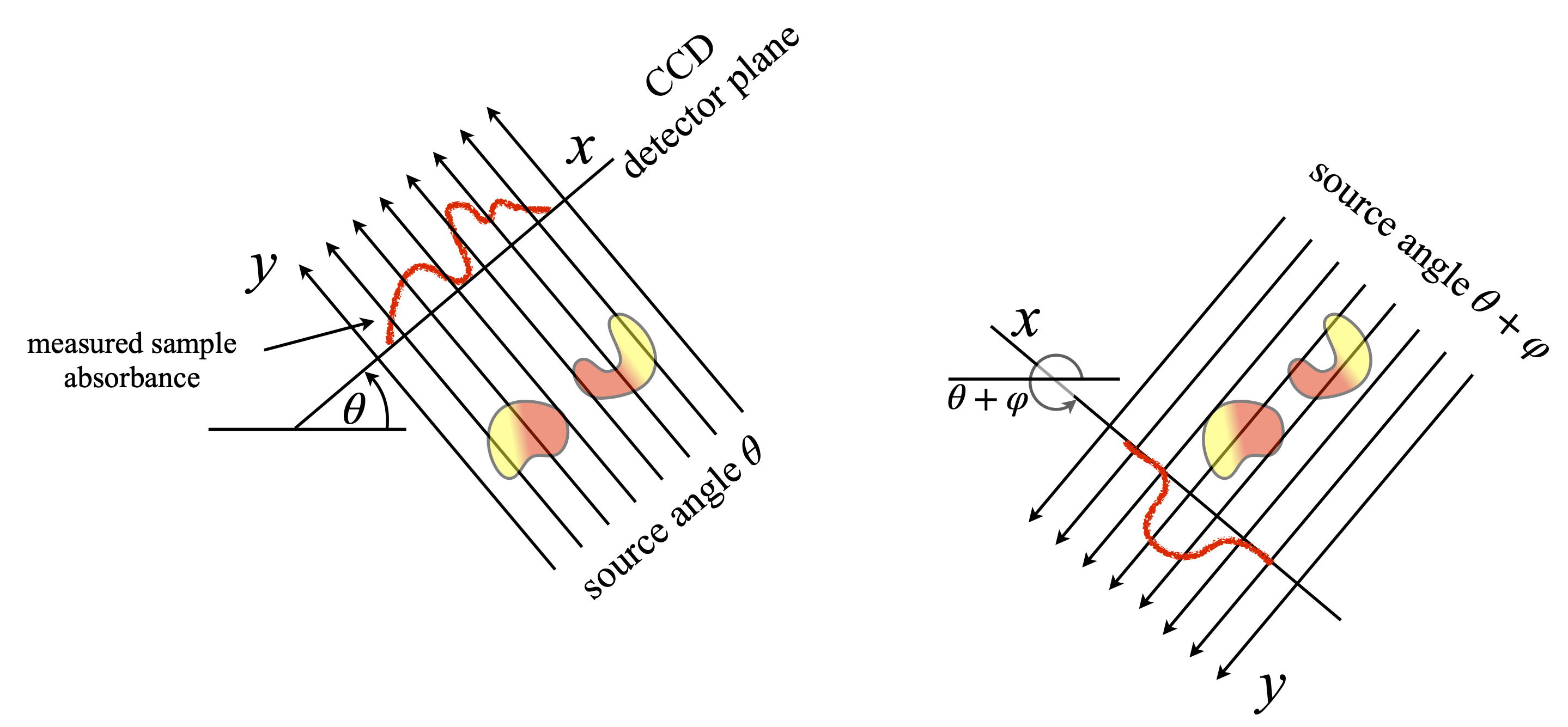
Figure 86. Two views of the same object, illustrating the necessity to measure at many angles. The measured absorption on the right would suggest that only one object is present. Hundreds of angles are measured over a \(180^\text{o}\) range as source and detector rotate as a pair about the object.
14.2 The Radon Transform#
In tomography we have to be far more general than in spectroscopy because absorption is not from one species at a fixed concentration. Additionally for each ray in the sheet of x-rays emerging from the source, the path length and absorption is normally different because these depend on the shape and nature of the object being measured. Thus, the Beer Lambert Law law is generalised and for each ray passing through the sample is at each angle is,
where \(f(x,y)\equiv \epsilon_\lambda [C]\) at position \((x,y)\) and the integration is over the ray’s path, \(y\) at each angle \(\theta\). The function \(p(\theta,x)\) is the projection of the total (i.e. summed) absorption onto the detector along path \(y\) at each horizontal position \(x\). In a spectrophotometer this would be called the optical density.
Mathematically, it is convenient to let each ray be defined by a perpendicular distance \(r\) from the origin and at each angle \(\theta\), see figure 87. The absorbance vs. position (see fig 86) clearly depends on the angle, but as the sample remains fixed in space there are two sets of coordinates to deal with. The first is the set belonging to the object being measured, the other that of the set of rays along with which absorbance is measured. The coordinates used are shown in figure 87. The object is positioned in the \((x,y)\) axes and the x-ray beam in the \((e_x,e_y)\) axes, a general point is labelled \((x',y')\). Integration along a typical ray occurs along the line \(R \to R'\), starting at \(I_0(\theta,x')\) at perpendicular distance \(x'\) from the origin and angle \(\theta\) and this produces a single absorbance value at \(p(\theta,x')\).
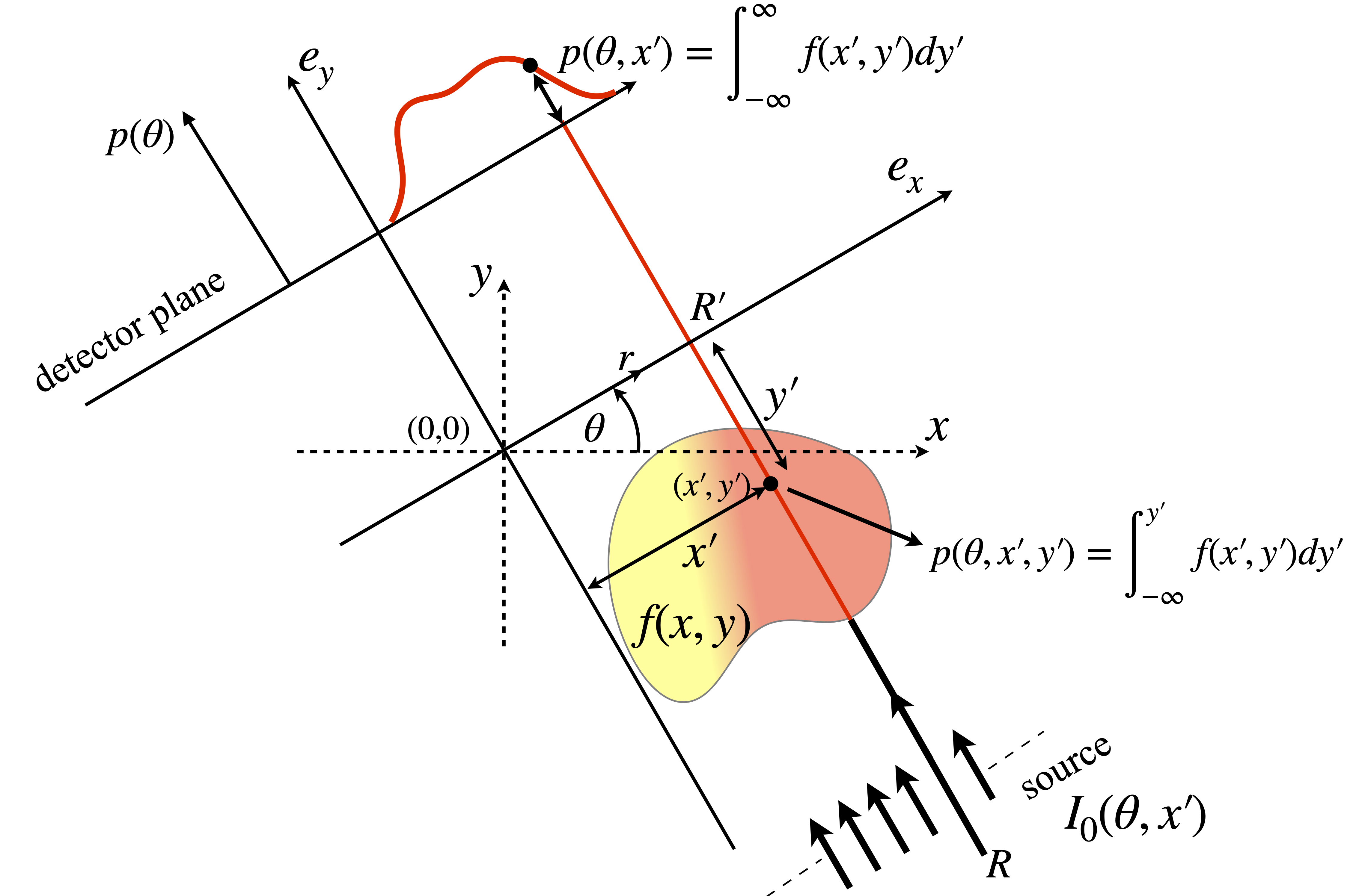
Figure 87. Details of the axes used. The total absorbance \(p(\theta,x')\) is that due to the whole path along \(y'\) at angle \(\theta\) and horizontal position \( x'\). The function \(p(\theta,x',y')\) is the absorption up to point \((x',y')\) at angle \(\theta\). A series of \(P(\theta,x')\) is recorded over a \(180^\text{o}\) range by rotating source and detector about the object being measured.
As the sample and x-ray are on different axes (the sample is fixed but the x-ray source moves in an arc) it is necessary to represent the path taken by a ray with path \((\theta,x')\) in terms of \((x,y)\). The way to do this is to find the equation of the line describing the path \((\theta,x')\). A straight line has the equation \(y=mx+c\) which can also be written as \(ax+by=r\) as shown in figure 88, where \(a=\cos(\theta),\;y=\sin(\theta)\) and \(r\) the perpendicular distance from the origin which is length \(x'\) in fig 87. This form is in polar coordinates and is more convenient for our use.
As the same straight line is followed when integrating then \(p(\theta,x')\) becomes
and is a two dimensional integral because as we track along the line at the distance \(x'\) from the origin, both \(x\) and \(y\) vary. The \(\delta\) function picks out just the values that are zero, \(x\cos(\theta) +y\sin(\theta) = x'\), i.e. \(\delta(0)=1\) else \(\delta(\ne 0)=0\) and thus follow the line with displacement \(x'\). The \(p(\theta,x')\) is called the Radon Transform after J. Radon (1917. (Translated by P. Parks, in IEEE Transactions on Medical Imaging, 5(4): 170-176,1986).
In the transformed coordinates the integral is
The transformation comes from finding \(x',y'\) using the rotation matrix, i.e. inverting the \(2 \times 2\) matrix and multiplying out

figure 88. Definition of straight line as distance \(r\) from the origin and angle \(\theta\). In effect this re-defines the line in polar coordinates \((r,\theta)\).
14.3 Sinograms#
When many sets of \(p(\theta,x')\) are accumulated the first step in unscrambling the data is usually to plot \(p\) vs. \(\theta\) as columns and using a grey-scale to indicate the magnitude of \(p\) and so form what is called sinogram which is the all the Radon transforms stacked one above the other. This name does not arise, as one might expect, from the shape of the image but from the fact that it was originally used to image the sinuses in the skull.
To illustrate the sinogram, suppose that the object to be imaged consisted of just one point at \(x_0,y_0\) then \(f(x_0,y_0)=\delta(x_0)\delta(y_0)\) and so from eqn. 62
and for simplicity suppose that \(y_0=0\) then \(p(\theta,x')=\delta(x_0\cos(\theta)-x')\), and this point traces out a sinusoidal curve in a plot of \(\theta\) and \(x'\). In fig 89, two objects are used (left figure) and right a sinogram calculated. The image repeats itself after \(360^\text{o}\) but is continued in the figure to show this more clearly. In practice only \(0\to 180\) need be calculated as the other angles are found by symmetry.
The two objects are centred at \((90,100)\) and \((200,150)\) and when \(\theta =0\) the \(x'\) values are the same as the \(x\) coordinate for each object as shown by the two small black dots. When the two sinusoids cross the angle is such that the objects are in line as in the right-hand image of figure 86. In this situation the \(x'\) axis is at right angles to the line between the two objects, and in this example, \(\theta \approx 114^\text{o}\) from the vertical and is shown by the red dots. The maximum \(x'\) happens when the angle places the detector surface parallel to the line between the two objects after accounting for their size and is at \(\approx 30^\text{o}\).
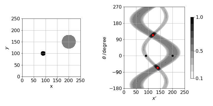
Figure 89. Example of a sinogram generated by two small objects on a \(256 \times 256\) grid. Angle \(\theta\) is defined in fig 87 vs. \(x'\), the distance along the detector surface.
14.4 Basic and filtered back projection.#
Once the sinogram is measured reconstruction is possible. The back projection method is currently very widely used to obtain the object’s image, see figures 90 & 91.
In back projection each row in the sinogram is in turn projected back (i.e. smeared, along the ray direction \(\theta\) that produced it) and then added to other projected rows rotated to their appropriate angle. What this means in practice is that a 2D square array is made with dimension of the number of pixels across the detector. The first row in the sinogram is (mathematically) smeared down this array, i.e. each row is made the same and the array rotated to the first angle in the sinogram and stored in another 2D array as the image plane. This process is repeated for each line in the sinogram and added to the stored image array. This forms the back projected image. Figure 90 shows as a schematic an initial object with two and then four back projections. As more of these are added the object becomes more defined. Figure 91 shows the calculated back projection forming an image of the objects in figure 89. In the projection the signal where the lines cross becomes large, but remains small at the perimeter where images overlap less. However, because the lines are placed radially, near to the centre the summed signal becomes blurred as there are so many of them adjacent to one another and so they still partially overlap where there should be no image. This effect diminishes towards the perimeter and is called the \(1/r\) effect. This is a convolution of the transform of the true object \(F(x,y)\) with \(1/r\) where \(r\) is the radial distance from the centre of the image. By rearranging the way the back projection is handled this effect can be counteracted in the ‘filtered’ back projection method described shortly.

Figure 90. To make a basic back projection of an object two then four ‘back’ projections are rotated then added together. The image becomes more clearly defined as more projections are added, but is far from being correct with just four projections. In practice many are needed as shown in the next figure.
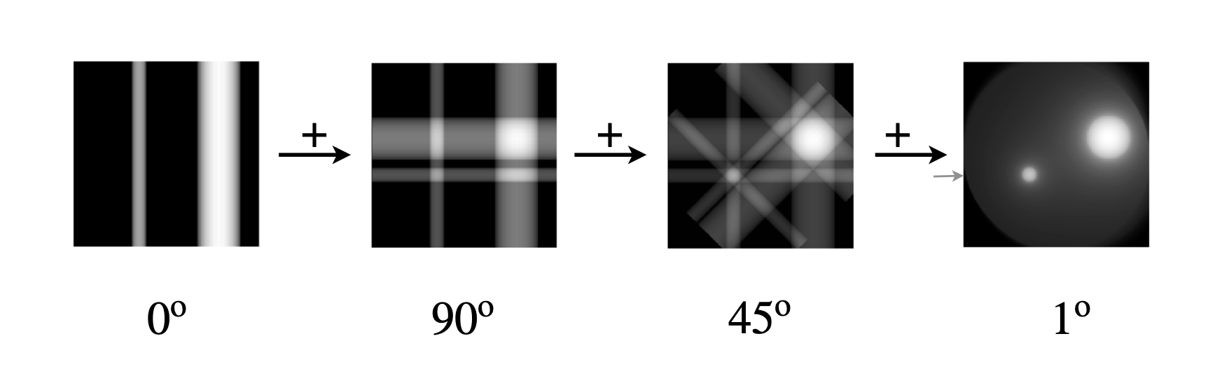
Figure 91. Calculated basic back projections using the image on the left of figure 89. Starting at the left the line of the sinogram at \(0^\text{o}\) is smeared along the whole of the image plane. In this example the image is \(256 \times 256\) pixels. The next image shows the smearing of this line added to a second at \(90\), the other images corresponding to lines at \(45\) and then finally at \(1\) degree intervals. The image is clearly reconstructed but is fuzzy with a undesirable diffuse halo around each feature. The small arrow shows the \(100^\text{o}\) object shown in fig 93, line B. (Rotating each 2D array is the most time consuming part of the calculation as it has to be done pixel by pixel unless an inbuilt function is used to do this. In python/scipy \(\mathtt{ndimage.rotate()}\) will do this rapidly.)
To understand why the reconstructed image is fuzzy the back projected image of a single pixel is shown in profile in figure 92. Clearly there is blurring because this should be a single spike and as the same thing happens to every pixel that is not zero, we can understand why the raw back projection is blurred the way it is. In optics this single pixel profile would be called the point spread function and as the point that generates it is cylindrically symmetrical the function spreads out in \(x\) and \(y\) in the same way. In figure 92 (right) the same x-ray intensity passes through areas A and B. The area A is \(r_1dr\delta\theta\) and B, \(r_2dr\delta\theta\). The intensity is energy/area or \(E/r_1dr\delta\theta\) and \( E/r_2dr \delta \theta \) which means in the general case that the intensity \(I(x,y)\sim 1/r\) as described above.
Another way of thinking about the blurring is to imagine the image as made up of a series of spikes that is convoluted with the point spread function. In this case to obtain the true image the blurred image needs to be convoluted with the ‘inverse’ function of the point spread function. However, as convolution is the same as multiplication in fourier space it is quicker to transform the image and multiply by the transform of the correction to the point spread function. How this is done is described next.

Figure 92. Left The raw back projected profile of a single pixel. Right. To show that the intensity profile is described as \(I(x,y)\sim 1/r\) where \(r\) is the radial distance. The centre of the image (point \(128,128\) in the images used here) is taken as \(r=0\).
While it can be appreciated by drawing pictures that the back projection will reform something that looks like the original object, at least approximately, it is important to check if this is always going to be the case or whether it may fail in certain circumstances. We start by looking at the inverse 2D fourier transform of a general object \(f(x,y)\), see equation 60, and finally arrive at the filtered back projection equation. In other words, by analysis a correction to the simple back projection is naturally produced.
As a reminder the 2D function of value \(f(x,y)\) at position \(x,y\) is, in effect, an image. The position \(x,y\) in ‘normal’ space will be called \(u,v\) in transform space, and by analogy with 1D transforms, the 2D transform is,
where \(u,v\) are the conjugate variables to \(x,y\), i.e. if \(x,y\) are in distance \(u,v\) are in reciprocal distance and so may be called the ‘spatial frequency’ but in tomography is called the projection. The \(1/\sqrt{\pi}\) scaling of the transform can be ignored. Examples of other 2D transforms are given in section 12.
The inverse 2D transform is
and we change this to polar coordinates i.e. to the (spatial) frequency domain with coordinates \(\theta, \omega\) where \(u = \omega\cos(\theta),\;v=\omega\sin(\theta)\). To find \(d\omega d\theta\) a Jacobian is used
making \(dudv=\omega d\omega d\theta\) and equation 66 becomes
Using the Slice Theorem (details below) the 2D transform \(F(u,v)\) can be replaced by the 1D transform at \(\theta\) of the experimental data which is the projection, \(P(\theta,\omega)\) which is a line in the sinogram. This is what connects the measured projection data to the true object \(f(x,y)\)
To get limits \(0 \to 2\pi\) the integral is split into two parts \(0\to\pi\) and \(\pi\to 2\pi\),
which may be simplified because \(\cos(\theta+\pi)=-\cos(\theta)\) and similarly for sines which changes the sign in the exponential, consequently, \(P(\theta+\pi,\omega)=P(\theta,-\omega)\) and the result for filtered back projection is
The \(|\omega|\) that arises in these last equations, as a result of changing to polar coordinates, is in effect a filter function and has a ‘V’ shape centred at the origin. It can account for the fact that there are too many points near to the origin compared to farther out, because the transform is arranged radially. The result of the radial arrangement is that the large values in frequency space, which correspond to small features (i.e fine details) in the image and not well resolved, therefore to improve resolution data at many angles are needed. This \(1/r\) blurring is removed by the filter \(|\omega|\), in other words the transform of the \(1/r\) in ‘real’ space is is \(|\omega|\) in transform space, thus we can easily perform the convolution, via fourier transforms, to remove the distortion caused by simple back projection.
Having measured the projections at all angles the filtered back projection method starts with the sinogram.
\(\quad\)(a) Fourier transform the first line in the sinogram.
\(\quad\)(b) Multiply this transform by the absolute value of the frequency (the filter function).
\(\quad\)(c) Calculate the reverse transform.
\(\quad\)(d) Continue to do this for all lines in the sinogram.
\(\quad\)(e) Construct the image plane with the new sinogram just as in normal back projection.
In practice the transforms have to be done numerically on a grid of data points and thus fast fourier transforms are used. The stages of the reconstruction are shown at the end of this section. Also the image can be constructed ‘on the fly’ rather than as suggested in (a)-(e) above. There are other concerns also, for example the filter \(|\omega|\) has to end at some finite value so has the form not of a V shape but more like an M and this introduces some extra frequencies as noise into the transform. Thus it is common to add some apodizing function by applying other filters (Gaussian, Hanning) to damping out these oscillations. Thus there is a trade-off between sharp edges to the image and some noise, vs. smoothing edges and less noise.
The image below shows the effect of filtering when compared to the right-hand most image in figure 91 which is basic back projection. The sharp edges are clear. The plot below shows the profile at \(100\) and \(150^\text{o}\). The wide blue line is the unfiltered back projection, and the increased precision by filtering is very clear. In this image only \(180\) projections were used and in the larger disc some of the remaining noise can be seen.
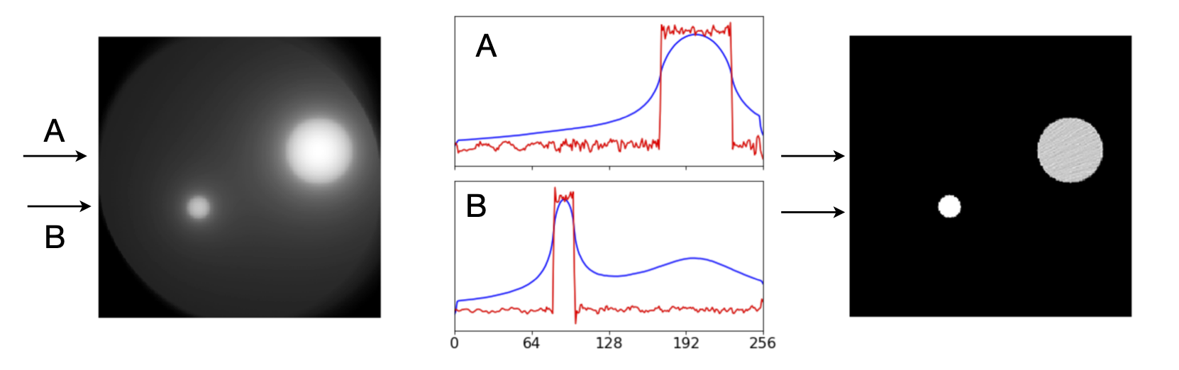
Figure 93. Left. Reconstruction of the object in figure 89 with basic back projection (left) compared with filtered back projection (Right). Middle, comparison of the profile along the line A (top) and along B (lower) for filtered, red, and basic back projection, blue.
14.4 Number of samples#
In practice discrete sampling has to be performed, both in terms of the number of pixels on a camera and in the angular resolution that is possible. As an example of the number of samples required to reconstruct an object \(f(x,y)\) let the minimum sampling distance be \(\Delta k_{max}\) which is defined in terms of the extent of \(f(x,y)\) and if this is \(\pm f_{max}\) then \(\displaystyle \Delta k_{max}=\frac{1}{2f_{max}}\), but \(\Delta k_{max}\) is also the product of the minimum angular separation and maximum spatial frequency as \(\Delta k_{max}=\Delta\theta \omega_{max}\). The maximum spatial frequency is \(\displaystyle \omega_{max}=\frac{1}{2\Delta x}\) and therefore
If there are \(1024\) pixels in the CCD detector then \(2f_{max}=1024\Delta x\) and so \(\Delta \theta =1/512\). As the total angular spread is \(180^\text{o}\) then the number of projections needed for an image of \(1024\times 1024\) pixels is \(N=\pi/\Delta\theta= 512\pi\approx 1600\) projections or at \(\approx 0.11^\text{o}\) intervals.
14.6 The Fourier Slice Theorem.#
The Fourier Slice theorem is used in the reconstruction as it allows the 2D image to be assembled from the 1D data. By transforming the projection \(p(\theta, x')\), one line of the 2D transform of the image is produced at angle \(\theta\). Repeating this at each angle and smearing and adding these 1D transforms forms the full 2D image as in back projection.
The fourier transform \(F(\cdots)\) of any \(p(\theta,x')\) will produce a new function \(P_\theta(\omega)\) in coordinates in reciprocal \(x'\) which we will label \(\omega\) as it is a ‘spatial frequency’. As the absorption is at fixed \(\theta\) this is a constant in the equations below. Fourier transforming one line of data \(p(\theta,x')\) gives
where the \(1/\sqrt{2\pi}\) scaling used in the definition of the transform (section 6) can be ignored. The next step is to relate this equation to the shape of the object \(f(x,y)\) and for this the Slice Theorem is used. ( As the fourier transform is used it is essential that the values at the limits of \(x'\) are zero, and this is because it is implicit in using the transform that the signal is repetitive and making values zero ensures that there is no sudden jump in values, which would present itself as as a artificial frequency. Zero padding would be used in practice to eliminate this effect if the values are not zero).
To illustrate the Slice Theorem and in its simplest form we start with the definition of the 2D fourier transform eqns. 65-66 but let \(v=0\) producing,
This integral can now be split into parts in \(x\) and \(y\), viz,
where the integral in the square brackets is the projection with \(\theta = 0\), i.e. \(p(0,x')\), from equation 62,
where in the last step we changed \(x' \to x\) which is the projection at constant \(x'\). Substituting into eqn 66 or 67 we find
and then recognize that the right-hand side is just the fourier transform of the projection at \(\theta=0\). In our example \(u\equiv\omega\) so we can write
which is eqn. 65 at \(\theta=0\). Thus we find that the fourier transform of the projection is in fact just a slice of the 2D transform of \(f(x,y)\), thus rotating each projection the 2D transform can be built up.
In the general case at angle \(\theta\) starting with equation 62,
The delta function is \(1\) only when \(x\cos(\theta)+y\sin(\theta)=x'\) making it selective for certain values and the integral is simplified to
This now has the form of a 2D fourier transform as in eqn. 60, i.e. \(\displaystyle \int_{-\infty}^\infty\int_{-\infty}^\infty f(x,y)e^{\large{-2\pi i (ux+vy)}}dudv\),
and is the 1D fourier transform of that part of the image \(f(x,y)\) that lies on the line defined by \(u=x\cos(\theta),v= y\sin(\theta))\) and is the general form of the Slice Theorem.
14.7 Stages in the filtered back projection.#
The figures show some data, starting with line 30 of the sonogram (length 256 pixels), which is at an angle of \(42^\text{o}\). The second image (B) shows the fast fourier transform of A but rotated by half its length (128) to make the centre of the transform at the centre of the array. This is then multiplied by the filter \(|\omega|\) with frequency zero at the centre. You can see how this product changes the transform giving it an inverted look. Finally the inverse /reverse or back fourier transform is made and again rotated so that it is at the centre of the data. By making the first and last points in the filter equal to zero adds a long period sine wave to the data as can be seen in frame E, but over all the angles the phase of this sine wave varies and eventually exactly cancels out.
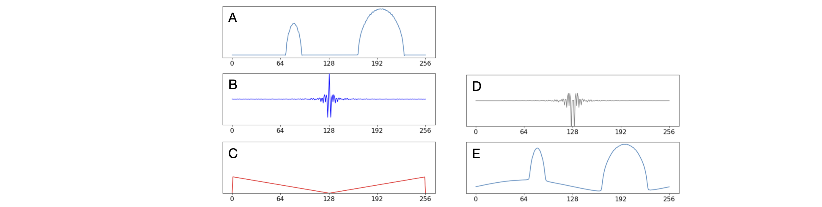
Figure 94. Showing stages in the filter back projection method. A; the sinogram at line \(30\) which is at \(42^{\text{o}}\). B; the real part of the fourier transform of A. C, the filter function \(|\omega |\). Zero frequency must be at centre point (\(128\)). D; the real part of (filter \(\times\) B). E; the back transform of D.
%matplotlib inline
import numpy as np
import matplotlib.pyplot as plt
from scipy import ndimage, misc
plt.rcParams.update({'font.size': 16})  # set font size for plots
# make the sonogram from the image call it p[ ..., ...], image is n by n.
# e.g n = 2**m to make FFT fast, say say 256
# This code is slow and not the most efficient but illustrates the method.

#----------------------------
def makeimage():

    image1 = np.zeros((n,n),dtype=float)

    x0a  = 200  # init values
    y0a  = 150
    rada = 30
    x0b  = 90
    y0b  = 100
    radb = 10

    for i in range(n):
        for j in range(n):
            image1[i,j]=0
            if (j-x0a)**2+(i-y0a)**2 <= rada**2:
                image1[i,j] = 20
            if (j-x0b)**2+(i-y0b)**2 <= radb**2:
                image1[i,j] = 40
        pass
    return image1
#----------------------------
def sinog(image1,n):                  # make sinogram

    p = np.zeros((n,n),dtype=int)
    for i in range(0,n,1):
        theta= (i*360/n)                        # angle degrees
        temp = ndimage.rotate(image1, theta, reshape = False)
        for j in range(n):
            p[i,j] = np.sum(temp[:,j])
    return p
#----------------------------
def filterproj(p):

    imtest = np.zeros((n,n),dtype = complex)      # image plane
    imk =    np.zeros((n,n),dtype = float)        # temporary storage
    temp=    np.zeros( n,   dtype = complex)      # temporary
    omega =  np.zeros( n,   dtype = complex)      # filter
    for i in range(n):
        omega[i] = abs(i-nc)                      # make centre zero
    omega[0] = 0.0
    omega[n-1] = 0.0
    for j in range(0,180,1):                      # jth  row of p
        indx = int(j*n/360)
        temp[:] = np.fft.fftshift(np.fft.fft( p[indx,:] ) )   # transform and shift to centre
        temp[:] = np.fft.fftshift(temp[:]*omega[:] )          # filter * transform, shift to edge
        temp[:] = np.fft.ifft(temp[:])                        # reverse transfer will auto shift back to centre
        for k in range(n):
            imk[k,:] =  np.real( temp[:]  )
        imtest = imtest + ndimage.rotate(imk, j, reshape = False)  # ndimage.rotate is fast array rotation
    return imtest
#----------------------------
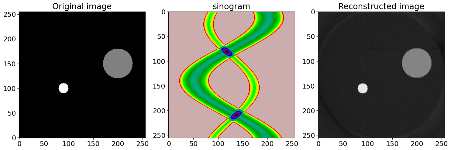
fig,(ax1,ax2,ax3) = plt.subplots( nrows=1, ncols=3, figsize=(15,10) )  # define plots

n = 2**8                                          # size of image to use
nc = n//2                                         # integer division

imageA = makeimage()
ax1.set_title('Original image')
ax1.imshow(imageA,origin='lower',cmap='gray')     # plot original image

p = sinog(imageA,n)
ax2.set_title('sinogram')
ax2.imshow(p, cmap='nipy_spectral_r')             # plot sinogram

fimage = filterproj(p)
ax3.set_title('Reconstructed image')
ax3.imshow(np.real(fimage) ,cmap='gray')          # plot filtered back transform

plt.tight_layout()
plt.show()