
Questions 24 - 37
Contents
Questions 24 - 37#
Q24 Operator#
If \(H_n(x)\) represents the Hermite polynomial, show that the operator
or equivalently
is true when the function \(f = 1\) by working out the first few terms then inferring the rest. Chapter 9.4 and Chapter 1.8.1 describe the Hermite polynomials.
Strategy: As \(D \equiv d/dx\) is an operator the order of multiplication is vitally important; for example, if \(a\) and \(b\) are operators then \(\displaystyle (a+b)^2 =aa+ab+ba+bb\) and \(ab\) may or may not be the same as \(ba\). The operator acts on the term to its right. An expression \(\displaystyle D^2f\) is the same as \(\displaystyle D(Df ) \equiv DDf \equiv d^2f/dx^2\).
Q25 SHM#
If a simple harmonic motion is described by \(x = A\sin(\omega t + B)\), and if the initial velocity is \(v_0\) and position \(x_0\) at \(t = 0\), find the amplitude \(A\) and phase \(B\).
Strategy: \(B\) is easier to find. Use the definitions of \(\tan\) and \(\cos^2(\cdots)+\sin^2(\cdots)=1\) to find \(A\).
Q26 Bodybuilder#
At the gym, a bodybuilder is lying on his back repeatedly pushing weights on a bar and doing so with a period of \(1\) s. If the bar is resting on his palms, what is the maximum amplitude displacement of the bar if it does not to leave his hands and assuming that the motion is simple harmonic?
Strategy: If the weight is not to leave his hands, then the maximum acceleration moving the bar must be no greater than \(g\), the acceleration due to gravity. The period \(T\) is related to the angular frequency as \(T = 2\pi/\omega\). Note that the weight lifted does not enter the final calculation.
Q27 Skidding bowling ball#
In a bowling alley, the ball and the surface of the alley are both smooth. This means that the ball can be made to skid until its speed slows enough that friction prevents this and the ball starts to roll and then does so at constant velocity (Lamb 1947). The ball has a mass \(m\), radius \(r\), and friction coefficient \(\alpha\) between the point of contact of the ball and the surface. The initial linear velocity is \(v_0\) and angular velocity \(\omega_0\). When \(v_0 \gt r\omega_0\) then skidding occurs and the frictional force \(\alpha mg\) opposes the linear motion, but when \(v_0 = r\omega_0\) the ball rolls.
(a) Write down two equations of motion for the linear and angular velocity assuming that the ball is skidding, and integrate them to find the linear and angular velocity. (It is convenient to use the moment of inertia as \(I = k^2m\) where \(k\) is the radius of gyration and write equations of motion as \(mdv/dt = \cdots\) and \(Id\omega /dt = \cdots\)).
(b) Next, assume that \(v = r\omega\) and find the time that the ball starts to roll and its linear speed. Show that \(v\) is independent of the friction coefficient but that the time is not. Explain these observations.
(c) Calculate the loss in kinetic energy.
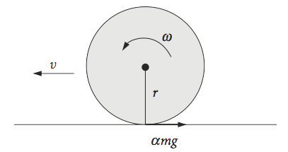
Fig. 18 A ball skidding/rolling on a surface with friction.
Strategy: Equate the linear force forwards with the negative value of the frictional force. Angular velocity is always calculated by using the moment of inertia instead of mass. The frictional force for the linear motion acts at the point of contact with the surface but with angular motion the frictional force is referenced to the centre of the ball so is a couple, i.e. the force times a distance, which in this case is the radius. The equations for linear and angular motion are independent of one another, and Euler discovered this in 1749 in connection with the motion of ships.
Q28 Inverse square force#
A particle is attracted with a force that varies inversely as the square of its distance from the origin.
(a) If \(\alpha\) is its acceleration at unit distance, write down and solve the equation describing the velocity at distance \(x\) from the origin of the force. Assume that the particle is initially stationary and starts at distance \(R\).
(b) Calculate the time taken to reach distance \(x\) from a very distant starting point \(R\) after starting from rest. Use the substitution \(x = R\cos^2(θ)\) to solve the integral. If at \(t = 0\), \(\theta\) = 0 and finally \(\theta = \pi/2\), calculate the time to reach the origin.
(c) Consider now that the ‘particle’ is the earth and that the earth’s orbital motion has been arrested. Using the last result, how long would it take the earth to fall into the sun given that the time of revolution in a circular orbit is \(t_c=2\pi\sqrt{R^3/\alpha}\) ?
(d) A meteorite is initially stationary and at a great distance from the earth, show that its velocity at the earth’s surface is \(\approx 11.2\,\mathrm{ km\, s^{-1}}\). This is numerically equal to the escape velocity.
(Notes: Assume no attenuation by the atmosphere. The constant in the force equation is now \(\alpha = gr^2\) where \(r\) is the radius of the earth and \(g\) the acceleration due to gravity. The acceleration due to gravity varies as the inverse square of the distance from the earth’s centre, where \(x = 0\). Assume that the initial distance of the meteorite \(R\) is very large making \(1/R\) negligible. The average radius of the earth is \(6371\) km and the earth - sun average distance is \(1.49 \cdot 10^8\,\mathrm{ km},\, g = 9.81\, \mathrm{m\, s^{-2}}\).)
Strategy: (a) As the velocity is required, use equation (16); the force is \(-m\alpha/x^2\) if \(x\) is the distance from the origin (centre of earth) and \(m\) the mass. (b, c) Use equation (15) to calculate the time. The substitution \(x = R\cos^2(\theta)\) greatly simplifies the integration. (d) The velocity is found when \(x = r\) at the surface of the earth. The starting point is so distant that the constant of integration can be set to zero.

Fig. 19 A small particle starts from rest at a distance \(R\) from a massive body.
Q29 Force inversely as distance#
A particle of mass \(m\) is moving in a straight line because it is attracted to a point with a force that is inversely proportion to its distance \(y\) from the point.
(a) Write down the differential equation for the force and integrate once to find the velocity \(dy/dt\) using the method of multiplying both sides by \(2dy/dt\). The constant of proportionality (force constant) is \(k\). The particle is stationary at \(y_0\) when \(t = 0\).
(b) Next, calculate the transit time taken to reach a distance \(y\) if the particle is initially at \(y_0\). Use the transformation \(y = y_0e^{-x}\) to simplify the integral. Show that this integral is the gamma function.
Strategy: Use ‘force equals mass times acceleration’. Find the time by inverting the velocity and integrating. The gamma function is defined as \(\displaystyle \Gamma (\alpha)= \int_0^\infty x^{\alpha -1}e^{-x}dx\).
Q30 Excited dimers#
When ground state molecules M are excited to an excited electronic singlet state M\(^*\), fluorescence may occur. If the solution is moderately concentrated, e.g. \(\ge 10^{-3}\,\mathrm{ mol\, dm^{-3}}\), then a ground state molecule may diffuse sufficiently to collide with an excited state before the latter has had a chance to fluoresce. In this case, an excimer or excited dimer can be formed and this species has an attractive potential well in its excited state (MM)\(^*\) but is repulsive in its ground state (MM). The reaction is
and the excimer (MM)\(^*\) can fluoresce but does so at longer wavelength than M* and its emission spectrum is broad and structureless, because the ground state is repulsive.
The interaction between M and M\(^*\) is caused by the combination of Coulomb and exchange interactions between the excited and ground state of the molecules. Excimers are formed with several types of planar aromatic molecules, pyrene being the most studied example (Birks 1970).
Excimer emission has found considerable use in determining the lateral diffusion coefficients of molecules in biological membranes. The rate of excimer formation is sensitive to the diffusion coefficient via rate constant \(k_d\) (see below). When the emission yield or, preferably, the time profile of the monomer and excimer fluorescence are analysed, \(k_d\) can be determined. Phase transitions, where viscosity may change suddenly can also be observed in this way.
Excimer and exciplex fluorescence can also be used to measure the proximity of one molecule to another, such as bases on complementary strands of DNA if they are suitably modified. If the two molecules are of different types, then the excited species is called an exciplex, short for excited complex. Partial charge transfer occurs between the two molecules in an exciplex therefore the emission is sensitive to the polarity of its environment and can be used as a probe of this. The two species in an excimer or exciplex need not be separate entities but can be linked to one another and, if this is long and flexible enough, intramolecular excimers and exciplexes can be formed.
The intermolecular excimer reaction scheme is
In this scheme \(E^* ≡ (MM)^*\) is the excimer concentration. The diffusion controlled rate constant is \(k_d\), the rate constant for monomer fluorescence is \(k_f\), and \(k_e\) is that for the excimer. Let \(M_0\) be the initial amount of \(M^*\) present at time zero and initially the excimer concentration is zero. As the number of excited species is small compared to the total, \(M\) is effectively constant making \(k_dM \equiv k_2\), a pseudo first-order rate constant. The reaction scheme is equivalent to a simple equilibrium;
(a) Describe what you would expect to see in an experiment to measure the time profiles of excimer \(E^*\) and \(M^*\) fluorescence.
(b) Solve the differential equations. Using the constants, \(k_f = 0.02, \,k_e = 0.01, \,k_2 = 10^{10} \cdot M_0, \,k_1 = 0.05\), each in units of 1/ns, and \(M_0 = 3\cdot 10^{-3}\,\mathrm{ dm^3\,mol^{-1}}\), plot the time profiles of \(E^*\) and \(M^*\) populations to see if your intuition in (a) was correct. Vary the rate constants and concentration to observe how the species respond. Initially \(E^* = 0\).
Strategy: Form a second-order rate equation from \(M^*\) and \(E^*\).
Q31 Electrical double layer#
The simplest model of a diffuse electrical double layer formed at an interface between an electrolyte in solution and a metal, a bilayer membrane, a protein or a colloid, consists of an excess of ions and electrons at the surface and an equivalent amount of oppositely charged ions randomly distributed in solution. This means that the electric field decreases more rapidly when moving away from the surface than would be the case in a vacuum.
The Poisson - Boltzmann equation describes the change in potential with distance and combines the Poisson equation of electrostatics with the Boltzmann distribution. In particular, the equation relates the time average of the space-charge density \(\rho\) to the potential \(\varphi\) at the interface. In one dimension, the equation has the form
and the charge density is
for \(i\) different species with charge \(z_i\). The boundary and initial conditions are that at \(x = \infty,\; \varphi \to 0\), and \(d\varphi/dx \to 0\). At \(x = 0,\; \varphi = \varphi_0\). The charge on the electron is \(e_0\) and \(\epsilon\) the permittivity or dielectric constant of the solvent.
Solve the equation and show that the electrical potential is \(\displaystyle \varphi = \varphi_0e^{-\kappa x}\) if the solution contains only a binary \(A^{z+}B^{z-}\) electrolyte with charges \(\pm z\) and \(N_i = N\) and simplify the final result of the integration assuming that \(k_BT \gg ze_0\varphi\). The constant is \(\displaystyle \kappa=\sqrt{\frac{8\pi Nz^2e_0^2}{\epsilon k_BT}}\).
(The double layer and Poisson - Boltzmann equation is described by Koryta et al. (1993), Kuhn & Fursterling (1999) and Jackson (2006)).
Strategy: Simplify the charge density first. Multiply both sides of the equation by \(d\varphi/dx\) and use the relationship
on the left hand side. See equation 14.
Q32 Series method#
Solve \(\displaystyle (1-x^2)\frac{d^2y}{dt^2}-2y=0\) by the series method.
Strategy: Use the \(n^{th}\) terms of the derivatives given in the text to work out the recursion equation.
Q33 Schroedinger equation with a rectangular energy barrier#
Particles with energy \(E\), such as electrons, interact with a rectangular one-dimensional energy potential barrier which extends from 0 to +\(a\), and has an energy height \(V_0\) and is zero elsewhere. The particles have a certain chance of being transmitted through or reflected off the barrier, the sum of these being unity.
(a) Write down the Schroedinger equation for the region inside the potential barrier.
(b) When \(E \gt V_0\) calculate the two wavefunctions \(\varphi_{1,2}\) which have an odd and even nature and are found with the initial values \(\varphi(0) = 0, \; d\varphi/dx |_0 = 1\) and vice versa.
(c) Show that the transmission is
and plot this vs. relative energy \(E/V_0\), with \(\sqrt{2mV_0} a/\hbar = 5\). To do this calculation use
with \(\displaystyle L_{1,2}=\frac{a}{\varphi_{1,2}}\frac{d\varphi_{1,2}}{dx}\). The \(L_{1,2}\) are then evaluated with \(x = a\).
The transmission is \(T=A^*_T A_T \); (* indicates the complex conjugate) use SymPy to do the algebra, and then use \(\displaystyle \sin^2(2x) = 4 \cos^2(x) - 4 \cos^4(x)\) or \(\cos(4x)=1-2\sin^2(2x)\) to simplify the result.
(d) Comment on the nature of the transmission vs. energy. What causes the oscillations?
(e) plot the transmission vs. barrier length and comment on the plot produced.
Strategy: Write down the standard Schroedinger equation with potential \(V_0\). It is easier to solve if you simplify using
Use the two conditions given to remove the arbitrary constants in the solution. To plot \(T\) vs reduced energy rearrange the transmission equation into terms in \(E/V_0\) then plot using this ratio as abscissa. You are given that \(\sqrt{2mV_0} a/\hbar = 5\).
Q34 Reaction and diffusion#
In example (iv) of Section 6.2 the diffusion out of a slab was calculated. Repeat this calculation, but now suppose that a reaction takes place so that the term \(-k_1c\) is added to the diffusion equation making it
The boundary conditions are that the concentration is \(c_0\) everywhere at \(t = 0\) and zero at the plate edges at \(t \gt 0\).
Strategy: Use the separation of variables method and base the solution on that of example (iv).
Q35 1D diffusion#
While it is possible to calculate the concentration profile of diffusing molecules, this is not usually measured, but instead the amount of material diffused out of a region as a function of time is measured. This quantity is
(a) Starting with the result of example (iv) shown in Fig. 24, which describes one-dimensional diffusion out of a slab, calculate \(c_{av}\) and then the ratio
where \(c_f\) is the final concentration determined by the boundary conditions, and \(c_i\) the initial concentration. Show that this ratio taken to long times is an exponentially decaying function.
(b) Suggest how the diffusion coefficient might then be measured.
Q36 Waveforms in a wire#
(a) Work out the waveforms produced if a taut piano wire of length \(L\) is struck such that its initial displacement is zero but its initial velocity everywhere has the shape \(f (x) = xL - x^2\).
(b) Show that the displacement is well approximated by \(\displaystyle u = 4\left(\frac{L}{\pi} \right)^3\sin\left(\frac{\pi ct}{L}\right)\sin\left(\frac{\pi x}{L}\right)\).
Strategy: Use the method outlined in the text. The integral for coefficients \(b\) can be solved; therefore, an algebraic series solution is possible. The integrals are
as can also be worked out by converting to exponentials.
Q37 Solitons#
A wave that retains its shape is not dispersive, this means that its wavelength does not change with time or distance, and is called a soliton. In the 1830’s, Russell published an account of his observation of a solitary wave travelling unaided along the Union Canal near Edinburgh. It was produced after a barge suddenly stopped but the mass of water it was moving did not. The same type of soliton wave is more famously observed as the Severn Bore. Solitons are also formed in some types of lasers and are important for communications, as the wave does not lengthen and one soliton can cross another unchanged. A soliton can also be formed in all-trans polyacetylene. In this case, it is an electron in a non-bonding orbital situated between regions of opposite double bond alternation. This electron density can migrate up and down the polyacetylene without spreading.
The Korteweg - deVries (KdV) equation
describes the motion of the classical soliton wave. The wave displacement at \(x\) and \(t\) is \(u\) and the shape of the wave is not unlike that of a Gaussian.
Show that \(\displaystyle u(x,t)= 3c\,\mathrm{sech}^2( \sqrt{c} (x-2at)/2 )\) is a solution of the KdV equation where 2\(a\) is the wave speed.