
Solutions Q7 - 10
Contents
Solutions Q7 - 10#
%matplotlib inline
import numpy as np
import matplotlib.pyplot as plt
from sympy import *
init_printing()                      # allows printing of SymPy results in typeset maths format
plt.rcParams.update({'font.size': 16})  # set font size for plots
Q7 answer#
(a) The fluorescence lifetime is \(\tau = 1/(1 \cdot 10^7 + 2 \cdot 10^8) =4.76\) ns. The yield is \(\varphi =k_f/(k_f +k_{isc})=k_f\tau =0.0476\), which is very small. The triplet state rises at the same rate as the singlet decays, i.e. in \(1/(4.76\) ns), not at the rate given by the intersystem crossing rate constant \(2 \cdot 10^8\,\mathrm{ s^{-1}}\). It is important to appreciate this.
(b) Algorithm 5 needs slight modification. The rate constants are different and the timescale needs to be changed to \(100\) ns, which is a guess, and may need to be changed later on. Because there are two reacting species, the excited state and the triplet, a check has to be made to make sure that the numbers in any of the states do not go below zero. Try the simulation with A0 = \(1000\) initial molecules in nA and increase these numbers as necessary. Eventually, the number of triplet states becomes zero and the calculation must end when this occurs because there are no more molecules left to react. At this point, the number in the ground state is equal to the initial number, and this is checked for in the ‘while nG \(\lt\) A0 do:’ step at the beginning of the loop.
The number of triplet states increase when populated from the singlet, and decrease when the ground state is reformed. Checks are needed to decide which reaction occurs, there are three, from the excited state to the ground state, to the triplet and from the triplet to the ground state adjusting the number of molecules each time as required. This involves several steps in the algorithm below.
The parameter \(a_0\), equation 8, is the sum \(a_0 =k_fn_A+k_{isc}n_A+k_Tn_T\). The rate constants must be put into a ns scale which means dividing \(k_k,\; k_{isc}\) by \(10^9\).
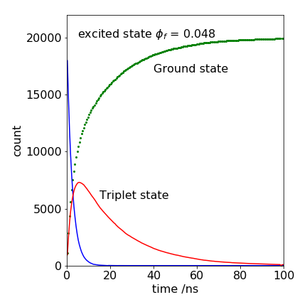
Figure 31. A Monte Carlo calculation of the decay of an excited state and the rise and decay of a triplet state, together with the increase of the ground state’s population. The parameters used are listed below.
# Algorithm: Gillespie Method rate equations S-> G, S->T, T-> G Q7 and figure 22

A0 = 20000
bins = 200
maxt = 100.0     # time in ns
kf   = 1e7/1e9   # in ns units
kisc = 2e8/1e9
kT   = 1/20.0
k1   = kf + kisc
phif = kf/k1     # fluorescence yield

Acount = np.zeros(bins,dtype=int)
Tcount = np.zeros(bins,dtype=int)
Gcount = np.zeros(bins,dtype=int)
dtime  = np.zeros(bins,dtype=float)

for i in range(bins):
    dtime[i]= maxt*(i+1/2)/bins   # work out time bins

G0 = 0                            # initial values
T0 = 0
nA = A0
nG = G0
nT = T0
t  = 0.0
Acount[0] = A0
Tcount[0] = T0
Gcount[0] = G0
indx = 0
while indx < bins and nG < A0 :   # check no negative counts
    a1 = k1*nA
    a2 = kisc*nA
    a3 = kT*nT
    a0 = a1 + a2 + a3            # summation eqn 8
    t0 = -np.log(np.random.random_sample())/a0  # equation 11
    t  = t + t0
    indx= int(np.round(t*bins/maxt))  # find bin number
    if indx < bins:
        r = np.random.random_sample()
        if r < a1/a0 :                # fluorescence chosen fraction a1/a0
            nG = nG + 1
            nA = nA - 1
            Gcount[indx] = nG
            Acount[indx] = nA
        elif r > (a1+a2)/a0 :         # triplet decay chosen
            nT = nT - 1
            nG = nG + 1
            Tcount[indx] = nT
            Gcount[indx] = nG
        else:                         # triplet formed chosen
            nT = nT + 1
            nA = nA - 1
            Tcount[indx] = nT
            Acount[indx] = nA
        pass
    pass
# plot time vs A , T and G populations
Q8 answer#
Modify the code for question 7. After setting the initial values inside the loop, the following changes can be made to account for the filling of state \(T\). The value of \(k_{isc}\) as it changes, is now called knT.
while indx < bins and nA > 0:
    if knT > 0:
        knT= 1.0 - 2.0*nT/A0
        k1 = kf + kisc*knT
    else:
        k1 = kf                # S -> triplet rate constn = 0
        pass

    a0 = k1*nA
    t0 = -np.log(np.random.random_sample())/a0
    t  = t + t0
    phif = kf/k1
The last statement \(\mathtt{phif = kf/k1}\) , is necessary inside the loop since this value changes as time proceeds. There are always two decisions to make; one calculates the time and the other which reaction will occur based on \(\mathtt{phif}\). At long times when the state T is full, the yield \(\varphi\) becomes unity because the state A can only convert to state G. If \(k_f\) is the fluorescence rate constant, then \(\varphi\) is the fluorescence yield, which is the same as the yield for ground state formation. The calculation should continue as long as nA does not become zero, and to ensure this, make its initial value equal to the number of events. The result of one simulation is shown below in Fig. 23.
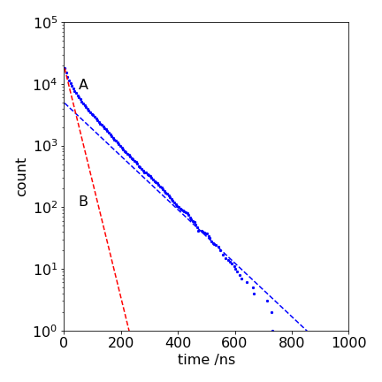
Figure 32. \(\log_{10}\) of the number of counts in the fluorescence signal (A), with the number of particles on the state T being restricted, and (B), with no restriction, giving the decay \(\exp(-(k_f + k_{isc})t )\). The dotted line following the data has a lifetime of \(1/k_f = 100\) ns, and the fluorescence reaches this value when state T is full.
Q9 answer#
The following modification to the Gillespie algorithm could be used. The whole calculation will need to be repeated, say, 100 times and the results averaged. This is because of the small number of individuals who could catch the disease and hence only a small number of trials are possible.
The average of the profiles calculated follows the expected pattern, although each time the calculation is done, it is a little different because of its random nature. The infected numbers rise and then fall; those susceptible to infection fall as they become infected and then immune, and enter the R or removed group.
# Algorithm: Gillespie method for S-I-R scheme

# Decision loop inside any averaging loop
# SIR    see also 11.9
# S+I -> 2I  k1=ksi ,   dS/dt = -k2[S][I], dIdt = +k2[S][I] -k1[I] , dRdt = k1[I]
# I -> R     k2=kIR.
# set initial values, define arrays to hold results
# start averaging loop.

while indx < bins :
    r1 = k1*nI
    r2 = k2*nS*nI
    a0 = r1 + r2 + 1e-20                           # eqn10, prevent being zero
    t0 = -np.log(np.random.random_sample() )/a0    # eqn 11
    t = t + t0                                     # increment time
    indx = int(t*bins/maxt)
    if indx < bins :
        Scount[indx] = nS
        Icount[indx] = nI
        r = np.random.random_sample()
        if r > r2/a0:
            nI = nI - 1
            remov = remov + 1           # reaction 2
        else:
            nS = nS - 1
            nI = nI + 1                 # reaction 1
        if nI < 0 :    nI = 0           # check>0
        if nS < 0 :    nS = 0           # check>0
        pass   # end while indx
# save and averaage nI and  nS
# plot results
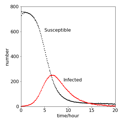
Figure 33. A Monte Carlo calculation of susceptible (S) and infected (I ) population in an S-I-R infection. The parameters used are given in the question and are \( k_2 = 2.18\cdot 10^{-3},\; k_1 = 0.452, \; S_0 = 762, \; I_0 = 1\).
Q10 answer#
Modifying algorithm in the text produces the following:
# main part of the Monte-Carlo method of evaluating
# Lotka-Volterra equations by the Gillespie method.

while indx < bins :
    r1 = k1*ny
    r2 = k2*nz*ny
    r3 = k3*nz
    a0 = r1 + r2 + r3+1e-20
    t0 = -np.log( np.random.rand() )/a0
    t = t + t0
    indx = int(np.trunc( t*bins/maxt ))
    if indx < bins :
        r = np.random.rand()
        if  r > ( r1 + r2 )/a0  :
            nz = nz - 1
            zcount[indx] = nz          # react 3
        elif r > r1/a0 :
            nz = nz + 1
            ny = ny - 1
            zcount[indx] = nz
            ycount[indx] = ny          # react  2
        else:
            ny = ny + 1
            ycount[indx] = ny          # react 1
            pass
        pass # end if indx
    pass     # end while  indx
Plotting the data, the populations oscillate as expected; one species grows at the expense of the other, which then almost dies off and then vice versa. See Chapter 11.7 for a fuller description. The fact that a Monte Carlo integration method is used means that the data is far more erratic than using an Euler integration method, just as might be expected because of random choices made as the calculation proceeds. Many more events would have to be taken to improve the result and to make it closer to a direct integration method. However, perhaps the result represents more closely what might happen in nature to two populations where there is only a limited number of individuals.
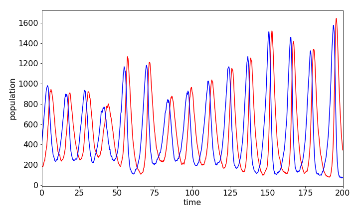
Figure 34. Predator and prey populations vs time calculated by the Monte Carlo solution of differential equations by the Gillespie method. Species \(Y\) (prey) is the blue line which rises before \(Z\), the red one, and always leads it. The parameters used were \(bins = 1000,\; maxt = 200.0,\; k_1 = 0.5,\;k_2 = 0.001,\;k_3 = 0.5,\;y_0 = 400.0,\;z_0 = 200.0\)