
Solutions Q35 - 40
Contents
Solutions Q35 - 40#
Q35 answer#
Use the shooting method algorithm described the text. The resulting curve is roughly U shaped crossing zero at \(\approx 3/4\) and having a minimum at \(\approx 3.4\). It is essential to modify the algorithm used to prevent division by zero such by adding a small term such as \(\approx 10^{-10}\).
Q36 answer#
Using the code,with a maximum \(x\) of 6, and an energy increment of 0.1, gives the results in table 4. A large value of \(x\) is essential to get accurate eigenvalues. Table 4 Calculated and theoretical eigenvalues of the potential \(V(x) = 10-10/\cosh^2(\alpha x),\; \alpha=1\).
Q37 answer#
Using a similar method to the previous question, with minimum energy 0 and maximum 10 the eigenvalues are shown in Fig. 48. The lower eigenvalues occur in pairs, as expected for a double well, and these are hardly separated at all in energy at small quantum numbers. When the potential becomes narrower, the levels interact more and their splitting becomes clear. Above the barrier, the levels separate from one another much as in the infinite square well.
Exercise: Investigate what happens when the barrier becomes very narrow and then very high and narrow.
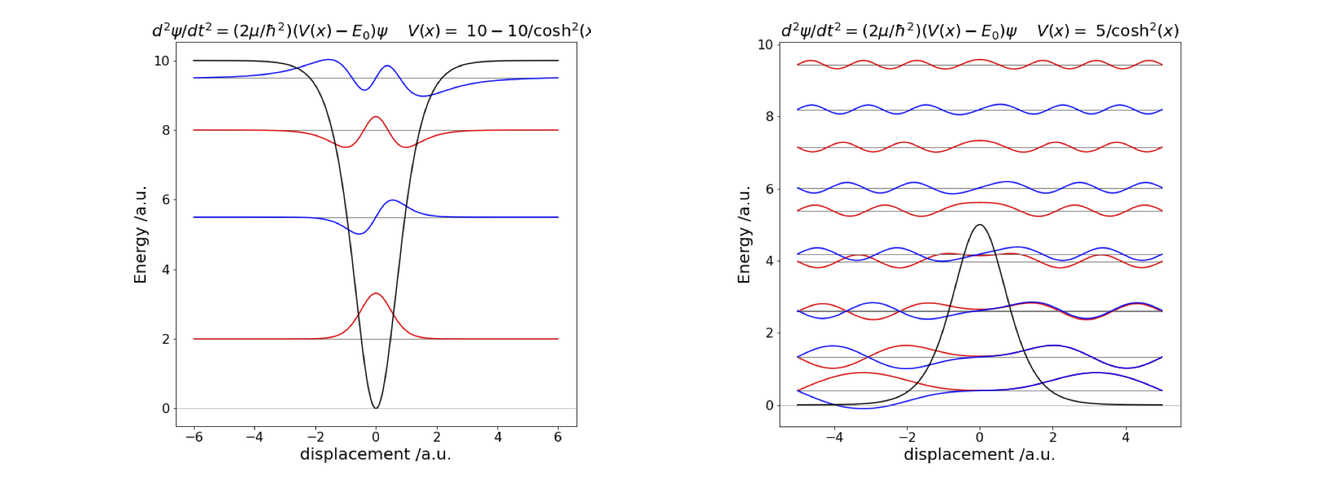
Fig. 48 Left: The potential well \(V(x) = -10/\cosh^2(\alpha x)\) , its four eigenvalues and wavefunctions. Right: The potential hill, \(V(x) = +5/\cosh^2(\alpha x)\) in an infinitely deep square well of width \(10\). The wavefunctions are for levels \(0, 1, 6, 7, 8, 9\) and \(10\).
Q38 answer#
Following the method outlined in Chapter 11.10.2, the only change is to the reduced mass making \(\mu/m_e = 4670.109\). The first four spectroscopic transitions are \(1.080, 41.02, 934.2, 976.3\). These values are better that when the ‘normal’ reduced mass is used. As it is derived from a more realistic model these values would be preferred.
(b) In ND\(_3\), using the normal definition of reduced mass \(\mu/m_e = 7694.3557\). The gaps between the energy levels compared to the experimental values are shown in the table. The experimental data is taken from Swalen & Ibers (1962). The agreement is quite good, particularly for the angle changed reduced mass. The significantly smaller splitting between levels is due to the heavier mass of D relative to H.
Q 39 answer#
Algorithm 20 in the text can be modified to use with these molecules. The parameters needed can be looked up in Herzberg (1950) but can also be found in textbooks.
Q40 answer#
The ionization energy of the H atom is, \(hcR_\infty = 13.6\) eV where \(R_\infty\) is the Rydberg. In atomic units, this energy is 1/2, which is 1/2 a hartree. In atomic units, the lowest level is at -1/2 and energies from -1 to 0 should therefore safely cover all numerical energies with an initial \(r\) value of 1 and an upper value of 100. Notice that as the energies reach zero when the quantum number \(n\) is large, they become ever closer together, as \(1/2n^2\), and in this case very small increments in energy will be needed not to miss the eigenvalues. Additionally, only the (even parity) initial conditions \(\psi (0)\) = 1 and \(\psi'(0)\) = 0, produce meaningful eigenvalues.
The data below shows the results, in hartree, calculated using the shooting method with the Numerov algorithm to calculate the wavefunctions and which also gave the best results.
It is clear that the eigenvalues are only approximately correct and illustrates that quantum calculations can sometimes be unexpectedly difficult.