
Solutions Q 43 - 73
Contents
Solutions Q 43 - 73#
# import all python add-ons etc that will be needed later on
%matplotlib inline
import numpy as np
import matplotlib.pyplot as plt
from sympy import *
from scipy.optimize import fsolve
init_printing()                      # allows printing of SymPy results in typeset maths format
plt.rcParams.update({'font.size': 14})  # set font size for plots
Q43 answer#
Starting with \(\displaystyle F_a =\left(\frac{\partial f }{\partial y}-\frac{d}{dx}\frac{\partial f}{\partial y_x} \right)\frac{dy}{dx}\)
multiplying and using the product rule gives, \(\displaystyle \frac{ \partial f}{ \partial y}\frac{dy}{dx}-y_x\frac{d}{dx}\frac{\partial f}{\partial y_x}-\frac{\partial f}{\partial y_x}\frac{d}{dx}y_x\)
and by cancelling terms and completing the differentiation gives, \(\displaystyle F_a=\frac{df}{dx}-y_x\frac{\partial^2 f}{\partial x \partial y_x}-\frac{\partial f}{\partial y_x}\frac{d^2y}{dx^2}\)
Expanding the second expression gives
The expressions \(F_a\) and \(F_b\) are the same if the term \(\displaystyle \frac{\partial^2 f}{\partial x\partial y_x}=0\) which will be the case if f does not explicitly depend on \(x\) because this term will be zero when differentiated by \(x\).
Q44 answer#
(a) Substituting produces \(\displaystyle f = x^2 + (e^{x^2})^2 + (2xe^{x^2})^3\)
then using the Chain Rule, \(\displaystyle \frac{df}{dx}=2x+4xe^{2x^2}+3(2xe^{x^2})^2(2e^{x^2}+4x^2e^{x^2})\).
(b) Differentiating \(x\) is straightforward. When differentiating \(y\), \(dy/dx\) is multiplied by the differential with respect to \(y\), which is \(\partial f/\partial y\), and the partial \(\partial\) is used to indicate that \(x\) and \(y_x\) are held constant. The same reasoning applies to the last term; the differential of \(y_x \)is
The result is \(\displaystyle \frac{df}{dx}=\frac{\partial f}{\partial x}+\frac{dy}{dx}\frac{\partial f}{\partial y}+\frac{d^2y}{dx^2}\frac{\partial f}{\partial y_x}\).
(c) Substituting terms from (b) using (a) gives \(\displaystyle \frac{df}{dx}=2x+2xe^{x^2}(2e^{x^2})+(2e^{x^2} +4x^2e^{x^2})3\left(2xe^{x^2}\right)^2\).
Imagine that \(y\) is any sensible function of \(x\) then use the function-of-function or chain rule, then for example, \(df/dy = 2e^{x^2}\) and similarly \(df/dy_x = 3(2xe^{x^2})^2\).
Q45 answer#
Using equation (32), and because \(x\) is not explicitly in the equation
Rearranging produces \(\displaystyle \frac{1}{\sqrt{1+y_x^2}}=const\), and therefore \(dy/dx = m\), where \(m\) is a new constant. Integrating produces the equation of a straight line \(y = mx + c\) and using the start and end points the gradient is \(m = (y_1 - y_0)/(x_1 - x_0)\) and the intercept is calculated by using similar triangles between the two points and the intercept (\(0, y\)). This produces \(\displaystyle y-y_0=\left(\frac{y_1-y_0}{x_1-x_0}\right)(x-x_0)\).
Q46 answer#
(a) The function is \(\displaystyle f=\frac{\sqrt{1+y_x^2}}{x}\). Using the Euler equation where \(\displaystyle \frac{\partial f}{\partial y}=0\) gives
Integrating with respect to \(x\) gives
where \(c\) is the integration constant. Solving this for \(y_x \equiv dy/dx\) produces
which can be integrated to find the path,
This integral has a standard form and can be looked up in tables or using SymPy gives
where \(d\) is the constant of integration.
The result using SymPy is
c, x = symbols('c, x')
ans = c*integrate( x/sqrt(1-c**2*x**2),x, conds='none')
ans

This result is the equation of a circle but does not look like it in this form but more so if rewritten as \(x^2 + (d y)^2 = 1/c^2\). The circle has a centre at ( \(0, d\) ) and radius \(1/c^2\).
(b) In this case \(f=\sqrt{x}\sqrt{1+y_x^2}\) and \(\displaystyle -\frac{d}{dx}\frac{\partial f}{\partial y_x}=-\frac{d}{dx}\frac{y_x}{\sqrt{x}\sqrt{1+y_x^2}}=0\). Integrating with respect to \(x\) gives \(\displaystyle \frac{y_x\sqrt{x}}{\sqrt{1+y_x^2}}=c\) and solving for \(y_x\) and integrating again produces \(y=2\sqrt{x-c^2}+d\) which is the equation of a parabola.
(c) The function is \(f = x\sqrt{ 1 + y_x^2}\), which produces, \(\displaystyle -\frac{d}{dx}\frac{\partial f}{\partial y_x}=-\frac{d}{dx}\frac{xy_x}{\sqrt{}1+y_x^2}=0\). Integrating in \(x\) gives \(\displaystyle \frac{xy_x}{\sqrt{1+y_x^2}}=c\) and solving for \(y_x\) gives \(\displaystyle \frac{dy}{dx}=\frac{1}{\sqrt{x^2-c^2}}\). This integrates to \(\displaystyle y=\ln\left(x+\sqrt{x^2-c^2}\right)+d\) where \(4d\) is the second integration constant.
Q47 answer#
The arrow below indicates separate differentiation top and bottom using l’Hopital’s rule, the = sign is there for rearrangement or substitution of the limit. Graphs of the functions can be sketched to confirm the limits.
(a) Nominally \(1/0\); so Hopitals’s rule does not apply as this is not an indeterminate form and the limit is infinity.
(b) Nominally \(0/0\); \( \displaystyle \qquad\lim_{x\to 0}\frac{x}{\sin(x)} \to \frac{1}{\cos(x)} =1\)
(c) Nominally \(0/0\); \( \displaystyle \qquad\lim_{\theta\to 0}\frac{\theta^2}{\sin(\theta)} \to \frac{2\theta}{\cos(\theta)} =\frac{0}{1}=0 \) because on adding limits after first differentiation this is no longer indeterminate.
(d) Nominally \(0/0\); \( \displaystyle \qquad\lim_{\theta\to 0}\frac{e^{-x}-1}{x^3} \to \frac{-e^{-x}}{3x^2}=-\infty\). After the first differentiation the result is \(1/0\).
(e)The limit is \(x \to -\infty\) and the product nominally \(-\infty \times 0\). To find the limit rearrange into a ratio, but trying this as
does not work because the powers of \(x\) are increasing and a constant will never be reached. Trying the other ratio gives
because \(e^{-x}\) is large when \(-x\) is large.
(f) \(\displaystyle \lim_{x \to \infty} x^{1/x}\) has the unusual form \(\infty^0\) and it is necessary to make this into a ratio. The way to do this is to take logs, find the limit and then convert back.
Taking logs gives \(\displaystyle \ln(x^{1/x}) =\frac{\ln(x)}{x}\) and taking the limit gives \(\displaystyle \lim_{x\to \infty}\frac{\ln(x)}{x}\to \frac{1}{x}=0\). However, this is the natural log of the limit of the initial function so that converting back by exponentiation gives \(\displaystyle \lim_{x\to \infty} x^{1/x} = e^0 = 1\).
(g) The expression has the form \(1^\infty\). Taking logs gives \(\displaystyle \tan(\theta)\ln\left(\sin(\theta)\right)\) which has to be put in the form \(\displaystyle \frac{\ln\left(\sin(\theta)\right)}{\tan(\theta)^{-1}}\). Differentiating gives
as this is the log of the expression the limit is therefore \(e^{0} = 1\). SymPy obtains the result directly.
x = symbols('x')
ans = limit( sin(x)**tan(x), x, pi/2 )
ans

(h) \(\displaystyle \lim_{x\to 0}\frac{e^{i\pi x}-e^{-i\pi x}}{ix}\to \frac{i\pi \left(e^{i\pi x}+e^{-i\pi x}\right)}{i} \to 2\pi\)
(i) This limit has the form \(0/0\) when \(\theta = 0\); but differentiating the cosines only produces a neverending ratio of sines and cosines but as \(\cos(n\theta) = 1\) when \(\theta = 0\) the limit is found. This can be confirmed by plotting the ratio.
(j) \(\lim _{x \to 0} x^x\) has the undefined form \(0^0\). Taking logs produces
and exponentiation gives the limit as \(1\).
(k) \(\lim_{n \to \infty} n!^{1/n}\) taking logs and using Stirling’s approximation for the factorial as \(n\) has to be large;
therefore in this case differentiation was not necessary.
(l) \(\displaystyle \lim_{n \to \infty}\frac{ n!^{1/n}}{n}\) taking logs and using Stirling’s approximation for the factorial produces the answer directly without the need for l’Hopital’s rule,
Q48 answer#
(a) Using l’Hopital’s rule, Section 7, \(\displaystyle \lim_{x\to 0}\frac{\sin(x)-x^2}{x}\to \frac{\cos(x)-2x}{1}\to 1\)
(b) \(\displaystyle \lim_{x\to 0}\frac{\left(\sin(x)+x\right)^2}{x}\to \frac{2(\sin(x)+x)(\cos(x)+1)}{1} =0\).
(c) This expression has to be made into a fraction to use l’Hopital’s rule. Multiplying by \(1\) using \(x+\sqrt{x^2 + x}\) allows completion of the square on the numerator. After differentiating, the limit at large \(x\) is taken to find the result.
The last step is not quite straightforwards and is made my expanding the fraction into
The last term here is zero as \(x\to \infty\), the middle term is \(1\) so the total is \(2\).
(d) In this case, the multiplier is \(x - \sqrt{x^2 + x}\) and the limit is infinity because the change in sign compared to (c) means that zero is produced in the denominator when \(x\) is large.
Q49 answer#
(a) Looking up \(\tanh\) and \(\cosh\) (Chapter 1.5.5) or elsewhere gives \(\displaystyle \tanh(x)=\frac{e^{2x}-1}{e^{2x}+1},\quad \cosh(x)=\frac{e^x+e^{-x}}{2}\).
Using l’Hopital’s rule, the limit at long time is
\(\displaystyle \lim_{t\to \infty} v_{\infty}\frac{e^{2gt/v_{\infty}}-1}{e^{2gt/v_{\infty}}+1}\to v_{\infty}\frac{2g/v_\infty e^{2gt/v_{\infty}}}{2g/v_\infty e^{2gt/v_{\infty}}}\to v_{\infty}\)
which shows that \(v_\infty\) is the limiting velocity because whatever the time taken to fall, and this is the fastest velocity achievable.
(b) The limit \(v_\infty \to \infty\) is calculated as
but this does not resolve into a constant upon further differentiation; the powers become larger. Instead substitute \(u = 1/v_\infty\) and the limit \(u \to 0\); this gives after differentiating by \(u\) top and bottom twice over,
Changing the cosh to its exponential form the limit on \(x\) is,
which means that the function must be differentiated twice to produce a constant on the denominator; \(u^2 \to 2u \to 2\). Using Sympy gives
u,g,t= symbols('u, g, t')
ftop = log((exp(g*t*u) + exp(-g*t*u)) /2 )
fbot = g*u**2
ans1 = diff(ftop,u) /diff(fbot,u)   # differentiate once  to and botton , limit still 0/0
ans1
ans2 = diff(ftop,u,u) /diff(fbot,u,u)   # differentiate top /bottom twice each
expand(ans2)

Using the expansion above, the limit \(u\to 0\) is \(\displaystyle \frac{gt^2}{2}\) and when \(v_\infty \to\infty\), \(\displaystyle x=\frac{gt^2}{2}\).
Q50 answer#
The limit is \(\displaystyle \lim_{x\to\infty}\frac{x^n}{e^x}\) which, using l’Hopital’s rule means finding the \(n^{th}\) differentiation of \(x^n\) before a constant is found on the numerator. This was worked out in Question 5 and is \(n!\); the limit is therefore \(\displaystyle \lim_{x\to\infty}\frac{x^n}{e^x}\to \frac{n!}{e^x}\to 0\) which shows that \(e^x\) is always larger than any polynomial \(x^n\) for any positive \(n\).
Q51 answer#
The substitution makes the function \(\displaystyle f=e^{-u^2}\) and its derivative
The limiting value where this derivative is zero is therefore \(\displaystyle \lim_{u\to\infty}\left(\frac{2u^3}{e^{u^2}}\right) \to \frac{6u}{2ue^{u^2}} = \frac{3}{e^{u^2}} \to 0\).
The second derivative is
and because both the function and first derivative are zero at \(x=0\), so is the second derivative. Using l’Hopital’s rule gives the same result.
and this will hold for any order of the derivative because, as shown in Q49, \(\displaystyle \lim_{u\to\infty}\frac{u^n}{e^u}\to \frac{n!}{e^u}\to 0\) any polynomial in the numerator produced by differentiation will never be larger than \(e^x\) and therefore the limit is always zero.
Q52 answer#
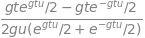
\(\displaystyle \frac{dy}{dx}=2x(x-1)^3+3x^2(x-1)^2\) and when the gradient is zero \(x\) has values \(0, 1, 2/5\). The second derivative is \(\displaystyle \frac{d^2y}{dx^2}=2(x-1)^3+12x(x-1)^2+6x^2(x-1)\). When \(x = 0\), this derivative is negative, so the point \(x\) = 0 is a maximum. When \(x = 1\) then the second derivative is zero as well as the first, so this is a point of inflexion, and by elimination \(x = 2/5\) should be a minimum. To prove this, the second derivative has the positive value \(18/25\). The function is plotted below. As an exercise find the maximum and minima of (a) \(y=|x^3|\) and (b) \(x\ln(x)\) over the range \(0 \to 1\).
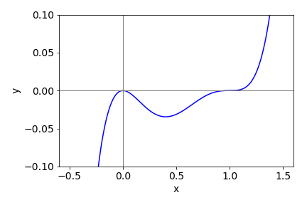
Figure 47. \( y=x^2(x-1)^3\)
Q53 answer#
Because the equation is given in parametric form, \(\displaystyle \frac{dy}{dx} = \frac{dy}{dt}\frac{ dt}{dx}\) must be used to calculate the derivative unless \(t\) is eliminated from the two parametric equations. This can be done but it produces a complicated result. The maximum occurs when \(\displaystyle \frac{dy}{dx}=\frac{dy}{dt}\left(\frac{dx}{dt}\right)^{-1}=\frac{\sin(t)}{1-\cos(t)}=0\).
Solving this equation produces zero at integer multiples of \(\pi\), or \(t = 0, \pi, 2\pi\), etc. Drawing the curve, Fig. 16, clearly shows that the maximum is at \(t = \pi\). The second derivative is \((\cos(t)-1)^{-1}\) which also confirms the maximum at \(x = \pi,\; y = 2\) when \(t=\pi\), assuming \(a=1\).
Q54 answer#
(a) The derivative is \(\displaystyle \frac{dy}{dx} = 2xe^{-ax^2} - 2ax^3e^{-ax^2}\) and should be set to zero to find any maxima or minima. The maximum and minimum \(y\) are found from \(\displaystyle xe^{-ax^2} =ax^3e^{-ax^2}\), which give \(x=0,\; x\to\infty\) or \(x=\pm 1\sqrt(a)\). To check that the last value is correctly chosen to be maximum value and not the minimum or a point of inflexion, the second derivative should be negative at this value. This derivative is
which is negative as \(a\) is positive.
(b) By examining the equation for \(P(u)\) it can be seen to have the same form as the example just studied if \(a=m/(2k_BT)\) and \(u=x\). The other pre-exponential term only contains constants. Therefore, substituting into the first derivative and multiplying by the constants produces,
and the maximum is at \(\displaystyle u_p=\sqrt{\frac{2k_BT}{m}}\).
The maximum speed is also the most probable speed, and using the data given this speed is, in \(\mathrm{m\,s^{-1}},\; 16.087\sqrt{T}\), or \(160.87\) at \(100\) K, \(278.63\) at \(300\) K, and \(359.72\) at \(500\) K.
(c) First,define the constants in SI units, putting mass \(m\) into kg. Let the speed distribution be a function of speed \(u\) and temperature \(T\). The python code below plots \(P(u)\) vs \(u\) at the temperatures shown
fig1= plt.figure(figsize=(9,4))          # set figure size
plt.rcParams.update({'font.size': 16})  # set font size for plots

amu = 1.6605e-27      # amu in kg
kB  = 1.3805e-23      # Boltzmann const J/K
m   = (32+2*16)*amu   # mass SO2 in kg

P = lambda u,T: (4/np.sqrt(np.pi))*(m/(2*kB*T))**(3/2)*u**2*np.exp(-m*u**2/(2*kB*T))

u = np.linspace(0,1000,200)     # set velocity range 0,1000 with 200 points
clr = ['red','blue','green']    # colours
for i,T in enumerate([100,300,500] ):
    plt.plot(u,P(u,T),color=clr[i])

plt.axvline(np.sqrt(2*kB*500/m),color='grey',linewidth=1,linestyle='dashed')
                                # plot vertical line at maximum of T=500
plt.ylim([0,0.006])
plt.annotate('100 K',xy=(125,0.0055) )
plt.annotate('300 K',xy=(250,0.0032) )
plt.annotate('500 K',xy=(500,0.002) )
plt.ylabel(r'$P(u)$')
plt.xlabel(r'$U \; /\,ms^{-1}$')
plt.show()
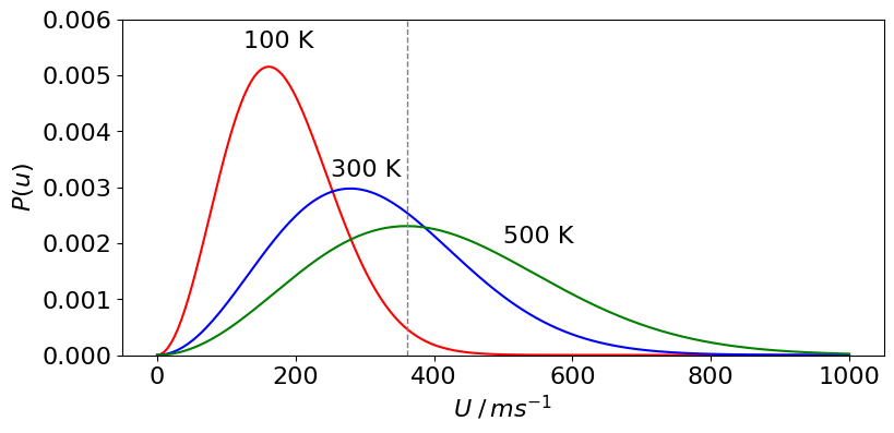
Figure 48. Maxwell - Boltzmann distribution at \(T = 1000, 300\), and \(500\) K for SO\(_2\). The vertical line shows the maximum of the distribution at 500 K.
(d) The distributions all have the same mathematical shape and the same area because the total probability, which is the area under the curve, must be 1. At higher temperatures, more molecules are moving faster than they do at lower temperatures, therefore fewer must be moving more slowly and the peak of the curve moves to higher speeds and is of smaller amplitude than at lower temperatures.
Q55 answer#
(a) Differentiating produces \(dy/dx = -2a/x^3 + 4b/x^5\) and at the minimum the gradient is zero, \(a/x^3 = 2b/x^5\) so that the one physically meaningful solution, if \(x\) represented a distance, is \(x = +\sqrt{ 2b/a}\). The other four solutions to the equation produce complex numbers, which cannot represent any physical distance.
(b) At the minimum energy, let the separation be \(r_e\) and here the gradient of the potential energy is zero and so
from which \(r_e = 2^{1/6}\sigma\) is the only possible solution. As \(2^{1/6} = 1.122\) the minimum separation is \(1.122 \cdot \sigma\) m or \(3.08\cdot 10^{-10}\) m very close to the experimental value of \(3.13\cdot 10^{-10}\) m.
The binding (minimum) energy is found by substituting with the minimum distance \(r_e\), and is \(-\epsilon /4\) or \(-0.775\cdot 10^{-3}\) eV.
Figure 49. The Lennard-Jones potential with parameters \(\sigma = 2.74 \cdot 10^{-10}\) m and \(\epsilon = 3.1\cdot 10^{-3}\) eV. The minimum is at \(r_e = 0.308\) nm.
Q56 answer#
Let ON be the distance \(x\) then as the area of a triangle is half the base times the height this is
To find the maximum, make the derivative of the area zero. You can take the derivative of \(A\) directly but because of the square root the result is complicated; to simplify the calculation take the derivative of \(A^2\) instead which is
and zero at the maximum or minimum, hence \(x = 1\) or \(4\) and if \(x = 1\) the maximum area is \((3/2)\sqrt{3}\). The second derivative is
and when \(x = 1\) this is negative because here \(dA/dx\) is zero and the area \(A\) is positive, therefore the maximum area is found when \(x = 1\).
You may also notice that \(x = 4\) is also a solution in which case the triangle is long and thin and produces the minimum area which must approach zero, see Fig. 17. To check the answer, sketch the change of area with \(x\).
Q57 answer#
To find the optimum, \(p\) has to be minimised with respect to \(v\) thus
from which \(\displaystyle v=\left( \frac{a}{3b} \right)^{1/4}w^{1/2}\).
Since \(w\) is weight this shows the necessity of reducing weight in an aeroplane but surprisingly only as its square root. To check this is a minimum, \(d^2p/dw^2\) should be positive at the calculated \(v\). Because
is clearly positive, both \(a\) and \(b\) being positive, the calculation has produced the optimum speed.
Q58 answer#
The gradient (tangent) is
and is zero when \(dy/dx=0\). Substituting for \(y\) produces
which has solutions at \(x = 0\), and \(x = \pm 3a/4\). The gradient would appear to be infinite at \(x = a\).
Q59 answer#
(a) First derivative: rearrange the equation to \(\sin(u) = p\), differentiating produces \(\displaystyle \cos(u)\frac{du}{dp}=\frac{1}{\cos(u)}\).
By differentiating again the second derivative is \(\displaystyle -\sin(u)\left(\frac{du}{dp} \right)^2 +\cos(u) \frac{d^2u}{dp^2} = 0\),
which simplifies to \(\displaystyle \frac{d^2u}{dp^2}=\tan(u)\left(\frac{du}{dp}\right)^2\).
As \(\sin(u) = p\), which is also defined as sine = opposite/ hypotenuse = \(p/1\) by the trigonometry of a right-angled triangle with a hypotenuse of 1, then, because the tangent is opposite/adjacent,
Substituting produces
(b) Generalizing, where \(f\) is any function that has an inverse, then \(f(u) = p\) and therefore by the ‘function of function’ rule
and differentiating again produces but now by the product rule,
Q60 answer#
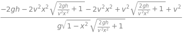
Making the substitution \(x=\sin(\theta)\) gives \(\displaystyle R=\frac{v^2x\sqrt{1-x^2}}{g}\left( 1+\sqrt{1+\frac{2gh}{v^2x^2}} \right)\).
The derivative is quite easily calculated by hand but is a long process; using SymPy it is,
x, v, g, h =symbols('x, v, g, h')

R  = v**2*x*sqrt(1-x**2)/g*(1+sqrt(1+2*g*h/(v*x)**2))
ans= diff(R,x)
simplify(ans)
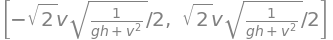
The maximum is found by solving the derivative when it equals zero.
xmax = solve(ans,x)
xmax
of which the positive solution gives the maximum value with \(x = \sin(\theta)\) at a given velocity. The surface of \(x\) vs speed \(v\) is shown in figure, together with the curve of maximum distance thrown. This is calculated by substituting \(x_{max}\) into the equation for the range \(R\) and evaluating \(R\) at each velocity; the \(45^\text{o}\) angled throw is also shown.
From the plot it can be seen that the throwing angle is small for slow throws and increases to about \(\sin(\theta) \approx 0.7\) or \(45^\text{o}\) only at very high launch speeds. About \(10\) m/s is about as fast as anyone can throw a football and the maximum distance for this throw has a launch angle of \(\approx 40^\text{o}\). For slower throws the launch angle should be smaller.
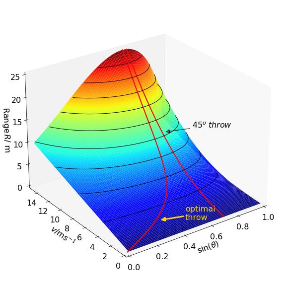
Figure 50 Throwing a football. The contours show the distance the ball travels and are separated by \(2.5\) m.
Q61 answer#
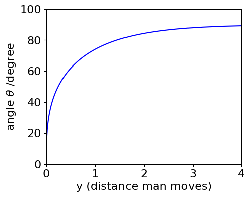
The angle is obtained from the tangent to the slope, which is the gradient \(dy/dx\). Differentiating both terms as a ‘function of function’ produces
which after simplification becomes \(\displaystyle \frac{dy}{dx}=-\frac{\sqrt{a^2-x^2}}{x}\). The angle is then \(\displaystyle \theta=\tan^{-1}\left(-\frac{\sqrt{a^2-x^2}}{x} \right)\) because \(\tan(\theta)=dy/dx\) but minus this angle is needed because of the way it is defined in the figure; a positive angle corresponds to a negative slope. When \(x=a\) the angle is 0o and when \(x=0\) it is \(90^\text{o}\).
To calculate angle as a function of the distance the man walks, it might be tempting to solve the tractrix equation for \(x\) and put this into the equation for the angle. However, solving for \(x\) is going to be very difficult and produce a complicated result, but is not necessary by plotting \(y\) vs \(\theta\) with \(x\) as a variable, i.e. plot parametrically. The python to do this is shown below
fig1 = plt.figure(figsize=(5,4))         # set figure size
plt.rcParams.update({'font.size': 16})  # set font size for plot

a = 1
x = np.linspace(1e-2,1,100)
y     = lambda x: a*np.log((a+np.sqrt(a**2-x**2))/x)- np.sqrt(a**2-x**2)
theta = lambda x: np.arctan(-np.sqrt(a**2-x**2)/x)

plt.plot(y(x),-theta(x)*180/np.pi ,color='blue')  # plot parametrically wrt x
plt.ylim([0,100])
plt.xlim(0,4)
plt.ylabel('angle '+r'$\theta$'+' /degree')
plt.xlabel('y (distance man moves)')
plt.show()
(b) The radius of curvature is \(\displaystyle \rho =\left( 1+\left(\frac{dy}{dx} \right)^2 \right)^{3/2}\left(\frac{d^2y}{dx^2} \right)^{-1}\).
Starting with the simplified version of the first derivative the second is \(\displaystyle \frac{d^2y}{dx^2}=\frac{a^2}{x^2\sqrt{a^2-x^2}}\) and substituting into the equation gives \(\displaystyle \rho = \frac{a\sqrt{a^2-x^2}}{x}\).
(c) The arc length \(s\) of any curve is defined as
Substituting for the gradient and simplifying gives
This integration is standard (see Chapter 4 Integration) and the result is \(s = a\ln(b/a)\) where \(a\) and \(b\) are points on the x-axis.
(d) If the dog is initially at \(x=a\), where \(a\) is the length of the lead given as one metre, then the distance the dog is pulled if the man walks 10 m is \(s = \ln(b)\), where \(b\) is the position on \(x\) when \(y\) = 10. This is obtained by solving for \(x\) with \(\displaystyle 10=a\ln\left( \frac{1+\sqrt{a^2-x^2}}{x} \right) -\sqrt{a^2-x^2}\).
Plotting the function, since this equation is not solved easily, produces a very small value for \(x \approx 3.3 \cdot 10^{-5}\) m, and so the distance travelled is \(\approx 10.32\) m. The Newton - Raphson method; see Section 10 could also be used to solve the equation more exactly. The minimum work done to pull the dog if it is a dead weight of \(25\) kg, is \(10.32\cdot 25 \cdot g = 2.53\) kJ, where \(g\) is the acceleration due to gravity.
Q62 answer#
(a) The mass/unit length of the bone is the mass of the bone plus that of the marrow; this is volume\(\cdot\) density, \(m = \pi r^2(1 - k^2)\rho + \pi r^2k^2\rho/2\). Rearranging and substituting for the radius in terms of the strength of the bone gives,
and differentiating, taking great care with the term in \(2/3\) power, then setting the result to zero gives,
Because the derivative is zero the constants cancel, and dividing by \((1 - k^4)^{-5/3}\) and also by \(k\) produces,
and simplifying produces \(3-8k^2+k^4=0\), and, remarkably, this equation is independent of the material’s properties \(Y\) and \(M\). Using Python to solve this equation produces
# must include fsolve using from scipy.optimize import fsolve
eqn = lambda x: 3  -8*x**2 + x**4
ans = fsolve(eqn,0.5)
print('{:s} {:6.3f}'.format('k value at minumum =', ans[0]) )
k value at minumum = 0.628
where \(k\) is the ratio of marrow to bone, (zero being solid bone), therefore, \(k \approx 0.628\).
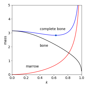
Figure 51. Mass/unit length of bone vs parameter for marrow \(k\), showing that the optimum is at about \(k = 0.63\). The total bone mass (see equation for \(m\) above) is plotted with separate curves for bone alone and marrow alone. The constants \(M,\; Y,\;\rho =1\). The dot show the minimum.
This simple model is very good at predicting the true value of the size of the marrow for mammal’s bones. Experimental values for the femur are, \(0.63\) for the fox, \(0.56\) in a lion, and \(0.62\) in the camel, but for birds, such as the swan, the value is \(\approx 0.9\), (Alexander 1996). This would seem to indicate that although a bone can be made with thinner walls it will break by buckling, like a drinking straw, instead of snapping. It is found that the swan has bones with internal struts to prevent buckling so that the simple model no longer holds and \(k\) is no longer meaningful.
The fact that the material properties of the bone do not enter the equation for the minimum mass vs \(k\) suggests that this is a universal behaviour to all animals. It would be interesting to see if this value for \(k\) is true for sea-dwelling creatures who experience different forces; one would expect that it is because the properties of the material cancel out in the equation for the minimum or optimum, value.
A comparison of bone with metals, such as stainless steel or aluminium, shows that for the same weight per length, bone is stronger than these metals but not as strong as carbon fibre composites.
Q63 answer#
Differentiating produces \(\displaystyle \frac{dI}{dJ}=2e^{-BJ(J+1)/k_BT}-\frac{(2J+1)^2B}{k_BT}e^{-BJ(J+1)/k_BT}=0\),
where \(k_B\) is Boltzmann’s constant. After cancelling terms and rearranging \(\displaystyle \frac{(2J+1)^2B}{k_BT}=2\) and solving gives
where the positive square root has to be taken since \(J\) cannot be negative. Finally, the numerical value of \(J\) should be rounded to a whole number because it is an integer.
Substituting values for HCl, \(J_{max} = \sqrt{k_BT/2 \cdot 10.58hc}-1/2\). To convert \(B\) into joules, multiply by \(c\) the speed of light in cm/s and by Planck’s constant. At \(100\) K, \(J_{max} = 1\) and at the same temperature for CO, \(J_{max} = 4\). The values at each temperature are shown in the table; notice the large increase in the maximum quantum number when the rotational constant is small.
Q64 answer#
(a) A maximum (or minimum) occurs when the derivative is zero, hence,
from which \(\omega = \omega_0\) at the maximum. The maximum, as might be expected, occurs when the applied radiation at frequency \(\omega\) is exactly at resonance. The derivative is also zero when \(\omega =\pm\infty\) and this is the minimum value of the function; when \(\omega \to \infty\) the 1 in the denominator is unimportant and because the power of \(\omega\) is larger here, and the function tends to zero.
The maximum has a value \(\tau/\pi\) and the fwhm the value when \(g(\omega)=\tau/2\pi\) gives \(\displaystyle \frac{1}{2}=\frac{1}{1+\tau^2(\omega-\omega_0)^2}\) and rearranging produces \(\omega=\tau^{-1}+\omega_0\), therefore the full-width is\(2/\tau\).
(b) The derivative has to be differentiated again to find the maximum and minimum. Although this can easily be done by hand, Sympy can help.
tau, omega, omega0, g = symbols('tau, omega, omega0, g')

g  = (tau/pi)*(1/(1 + tau**2*(omega - omega0)**2))
ans= diff(g,omega,omega)
simplify(ans)
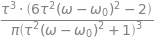
and as this result must equal zero then \(\displaystyle \omega = \omega_0+\frac{1}{\tau\sqrt{3}}\). The separation between maximum and minimum is therefore \(2/(\tau\sqrt{3})\).
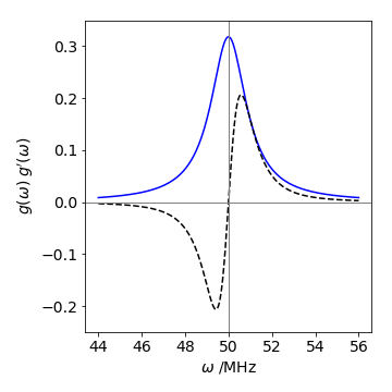
Figure 52 Lorenzian \(g(\omega)\) and its derivative \(g'(\omega)\)(dashed line); \(\tau = 1\) s, \(\omega_0= 50\) MHz.
Q65 answer#
(a) Differentiating \(\rho\) with respect to \(\lambda\) as a product and ‘function of function’ and setting the result to zero produces
Simplifying to find \(\lambda_{max}\) produces
In this equation \(\lambda_{max}\) appears on both sides, which is annoying because it makes it very hard to solve. A solution can be found numerically by iteration using the Newton - Raphson method. However, an approximate solution can be found, because, if \(hc/\lambda k_BT \gg 1\) the exponential term is then very small compared to \(1\) ( \(e^{-big}\) = small ) and can be ignored and this results in the approximation \(\lambda_{max}T \) = constant, or more precisely,
(b) To justify this approximation,the exponential term must be made small compared to unity; for example if \(hc/\lambda k_BT \ge 10\) then \(e^{-10} \approx 4 \cdot 10^{-5}\) and thus \(\lambda T\) needs to be smaller than \(1.4\cdot 10^{-3}\). Using values for Planck’s constant \(h\), the speed of light \(c\), and Boltzmann’s constant \(k_B\) then \(hc/k_B = 0.01439\). The wavelength \(\lambda\) for red light is around \(600\) nm and suppose \(T = 2000\) K, then \(\lambda T = 1.2\cdot 10^{-3}\) and our condition is just satisfied for visible light and relatively low temperatures for the black body. If the full equation for \(\lambda T\) is solved, then \(4.965\) replaces the constant \(5\) used in the approximate equation.
Q66 answer#
The probability of the nuclei being at separation \(x\) is \(\displaystyle \psi^2=\sqrt{\frac{\alpha}{4\pi} } (2\alpha x^2-1)^2e^{-\alpha x^2}\)
and therefore the maximum or minimum if found from the derivative
Cancelling the constants and excluding \(x \to \infty\) as being physically unrealistic, the exponential terms can also be cancelled then \(x\) is found by solving
and here there are five solutions as this is a fifth-order polynomial (because there are terms in \(x^5\)). By inspecting the equation one solution occurs when \(x = 0\), two when \(2\alpha x^2-1 =0\) or \(x=\pm\sqrt{1/(2\alpha)}\) and two by solving \(4-(2\alpha x^2-1)=0\) or \(x=\pm\sqrt{5/(2\alpha)}\). By plotting \(\psi^2\) the solutions make more sense; and the last one corresponds to the maximum as shown by the red dots on \(\psi^2\). The other solutions \(\pm\sqrt{1/(2\alpha)}\) correspond to the mimima and zero to a sub maximum.
Figure 53 The harmonic oscillator wavefunction \(\psi\) when \(v = 2\) and \(\psi^2\) on the same scale. The red dots show the position of the maxima, \(\pm\sqrt{5/(2\alpha)}\). The same calculation using SymPy is shown below. The solution generated has evaluated the square roots; \(1.581=\sqrt{5/2}\).
a,x = symbols('a, x')             # define symbols to use
psi = ( a/(4*pi))**(1/4)*(2*a*x**2 - 1)*exp( -(a/2)*x**2 )
ans = diff(psi**2,x)           # differentiate psi^2
ans

solve(ans,x) # solve equation

Q67 answer#
(a) Starting with \(f\), the derivative is
and substituting for \(dx/df\) gives
(b) Differentiating the equation for \(h\) given in the question produces \(\displaystyle \frac{dh}{df} = \frac{d^2x}{df^2}\),
which means that \(\displaystyle \frac{d^2x}{df^2}\) has to be found. To do this, start by differentiating both sides of the identity \(\displaystyle \frac{df}{dx}=\left( \frac{dx}{df}\right)^{-1}\) by \(x\) which produces
and because \(\displaystyle \frac{dh}{df}=\frac{d^2x}{df^2}\) therefore
which is the result sought.
Finally, using the derivative from part (a)
and all the terms in this expression are known.
Q68 answer#
(a) \(D_e\) is the dissociation energy, because when \(r \to \infty\) the potential \(V \to D_e\). The constant \(\beta\) has units of 1/distance because the exponential must be dimensionless.
(b) The potential energy and force are shown in Fig. 54. The derivative \(dV/dr\) equals force at any internuclear separation \(r\) because energy = force \(\times\) distance, therefore force is energy/distance or \(dV/dr\),
(b) At the minimum (or maximum ) of the potential energy the force is zero, see Fig. 54, which occurs when either \(r=\infty\) or \(e^{-\beta(r-re)} =1\) and the latter is true when \(r=r_e\).
The second derivative allows us to find the maximum force, and after some simplification this is
The maximum attractive force occurs when \(d^2V/dr^2=0\) and \(d^3V/dr^3 \lt 0\). One solution is found when \(r = \infty\), which is unphysical as any bond will have been broken; the other when \(2e^{-\beta(r-re)} = 1\) and therefore \(r_{max_f} = r_e + \ln(2)/\beta\). Notice that the force changes sign at the equilibrium internuclear separation to become repulsive (negative) at a shorter separation than this, and attractive at a larger separation, eventually dying away to zero as the atoms separate.
(c) Substituting values into this last equation the maximum force in the bond extension is at \(0.167\) nm or \(1.31r_e\) and by substituting this value into \(dV/dr\) the maximum force is \(7.4\) nN (\(1\) nN = \(10^{-9}\) N). This does not appear to be too much, but work it out per mole and the compare the force due to gravity you experience.
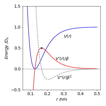
Figure 54 The Morse potential for HCl, in units of \(D_e\), the force, and the second derivative. By convention, zero energy is often placed when \(r = \infty\) on the potential energy curve. The force and second derivative are divided by \(\beta\) and \(\beta^2\) respectively to give energy. The dot shows the maximum force at \(r_{max_f} = r_e + \ln(2)/\beta\).
Q69 answer#
(a,b) The maximum number of levels is found when the difference in energy levels approaches zero then
and as \(x_e = 0.0174098, \,n_{max} = 28\). The calculated dissociation energy is \(E = 42928.8\,\mathrm{ cm^{-1}}\) or \(0.9994D_e\) , which is very close to, but just below, the dissociation energy.
(c) The calculation, assuming discrete quantum numbers, is shown below and in cm\(^{-1}\) for simplicity. The differences in the energy of the \(n^{th}\) and \((n + 1)^{th}\) terms are checked and as long as \(E_{n+1} \gt E_n\) the quantum numbers \(n\) are incremented.
nu = 2989.7
xe = 0.0174098
E  = lambda n: nu*(n+1/2) - nu*xe*(n+1/2)**2
n  = 0
while E(n+1) > E(n):
    n = n + 1
print('{:s} {:d}{:s} {:8.2f}'.format('n_max =',n, ', D_e =', E(n)) )
n_max = 28, D_e = 42928.77
This value is the same as by differentiation.
(d) Plotting the energy level differences \(\Delta E = E_{n+1} - E_n\) vs \(n\) produces a Birge - Sponer extrapolation which in this case extends to \(\Delta E = 0\). Unlike our ideal data, Fig. 55, if a real set of data points were used, there would have to be an extrapolation past the data to the x-axis, because real data rarely extends to the dissociation limit. The extrapolation is made to find the dissociation energy \(D_0\) from the zero point, not the bottom of the potential well, which would give \(D_e\). By plotting the energy difference against quantum number the dissociation energy is the area under the line.
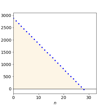
Figure 55. Dissociation energy \(D_0\) (from zero point) is the area under the curve of \(\Delta E =E(n+1)-E(n)\) vs quantum number \(n\).
Q70 answer#
(a) The equilibrium occurs when \(dG/d\xi =0\) and \(G\) is a minimum. The equation is best differentiated in two parts, then combined and simplified. Taking the first term,
and the second
Adding the two derivatives produces
At equilibrium, as the derivative is zero, simplifying the previous expression produces
This equation is, of course, just \(\Delta G^\text{o} =-RT\ln(K_p)\).
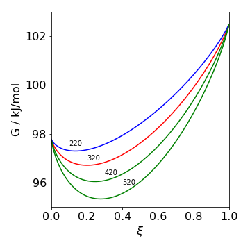
Figure 56. Free energy \(G\) vs extent of reaction \(\xi\) at the temperatures shown.
(b) Using the numerical values given, \(\displaystyle \ln\left(\frac{4\xi_{eq}^2}{1-\xi_{eq}^2} \right)=1.78\). The equation can be solved to find \(\xi_{eq}\) and the equilibrium constant \(K_p\). This can be done by hand and also numerically using python with scipy as follows
DeltaGN2O4 = 97.79*1000  # J/mol
DeltaGNO2  = 51.26*1000

R = 8.314  # J/K/mole
T = 320    # K
dDeltaG = lambda xi: 2*DeltaGNO2-DeltaGN2O4 + R*T*np.log(4*xi**2/(1-xi**2))

xi_eq = fsolve(dDeltaG,0.1)[0]    # 0.1 is initial guess, take 1st answer only with [0]
k_p   = 4*xi_eq**2/(1 - xi_eq**2)
print('{:s} {:6.4f} {:s} {:6.3f} '.format('xi(eq) =', xi_eq ,', K_p = ',k_p) )
xi(eq) = 0.2013 , K_p = 0.169
Q71 answer#
(a) The maximum \(P(t)\) occurs when the rate of change of \(P\) is zero. The derivative is
which is zero at
In the sample, the pheophytin signal grows as it receives the electron from (BChl)\(_2\) and decays as it transfers the electron to the quinine, thus passing through a maximum.
In the question the decay lifetime is \(2\) ps or \(k_c = 0.5 \cdot 10^{12}\) and \(k_p = 0.005 \cdot 10^{12}\,\mathrm{ s^{-1}}\), then \(t_{max} = 9.3\) ps and should be the best place to observe the spectrum as shown below.
(b) If the spectra of the two species overlapped, then a time such as 20 ps would be acceptable because the (BChl)\(_2\) has effectively decayed to zero but the BPh signal is still large.
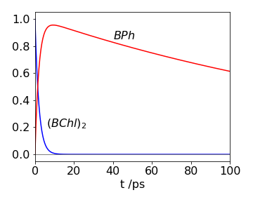
Figure 57. Time profiles of (BChl)2 and BPh populations.
Q72 answer#
(a) The minima are found by differentiating the potential with respect to angle and solving the resulting equation which means solving \(4\theta^3 - 14.4\theta = 0\). Note that the equation is a cubic, but one power of \(\theta\) can be cancelled and this gives us \(\theta = 0\) as a solution leaving a quadratic, which is then easy to solve. This produces \(\theta = 0\) and \(\pm 1.897\) radians or \(\pm 108.7^\text{o}\). The height of the barrier is the difference between the maximum and one of the minima, and by substituting for the angles, is \(2008.8\,\mathrm{ cm^{-1}}\). Notice that as the barrier is of finite size, the energy levels on one half of the potential are influenced by the others, and vice versa, leading to a splitting of the levels.
(b) The (smallest) number of inversions/second is the same as the lowest frequency, which is \(0.79\,\mathrm{ cm^{-1}} \cdot 2.9979 \cdot 10^{10}\, \mathrm{cm\, s^{-1}} = 2.37\cdot 10^{10}\,\mathrm{ s^{-1}}\) and is a period of \(\approx 42\) ps.The energy gap of the lowest level is caused by inversion and this, therefore, is the inversion frequency of that level.
Q73 answer#
The minimum is found from the derivative \(\displaystyle \frac{dE}{d\theta}=-2NS^2\left(-J_1\sin(\theta)-2J_2\sin(2\theta)\right)=0\).
This equation is satisfied if interactions (J’s) between layers are zero, which they are not, or if \(-J_1 \sin(\theta) = 2J_2 \sin(2\theta)\). There are therefore three solutions. The two most obvious ones are, \(\theta = 0\), making the crystal a ferromagnet and \(\theta = \pm \pi\), making it an anti-ferromagnet.
The third solution can be most easily seen by using the identity \(\sin(2\theta) = 2 \cos(\theta)\sin(\theta)\) then \(-J_1 = 4J_2 \cos(\theta)\). This third solution \(\theta = \cos^{-1}(-J_1/4J_2)\) causes helimagnetism; here the planes containing the magnetic moments are parallel to one another, but the magnetic moments are separated by the fixed angle \(\theta\) as in a helix.