1 Real, imaginary, conjugate and modulus
Contents
1 Real, imaginary, conjugate and modulus#
# import all python add-ons etc that will be needed later on
%matplotlib inline
import numpy as np
import matplotlib.pyplot as plt
from sympy import *
init_printing()                      # allows printing of SymPy results in typeset maths format
plt.rcParams.update({'font.size': 16})  # set font size for plots
1 Motivation and concept#
Complex numbers arise naturally in mathematics, often when solving quadratic equations such as \(x^2+x+1=0\), which has the solutions
Because the negative square root cannot be evaluated, as no ordinary number can be negative when squared, a new number conventionally called \(i\) (although engineers call this \(j\)) was invented with the property \(i^2 = -1\) or \(i = \sqrt{-1}\). The solution to the equation becomes \(x = 1/2 \pm i\).
This new number is one of a new class called complex numbers. These are not numbers in the elementary sense used in counting or measuring, but constitute new mathematical objects and have an existence of their own. These numbers are called ‘complex’ only because they contain two parts and can always be written in the form
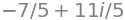
where \(a\) is called the real (Re) part and \(b\) the imaginary (Im) part of the number. The complex number \(z = i\), if written in the form of equation 1, has a real part \(a = 0\) and an imaginary part \(b = 1\). The latter is rather a misnomer as \(b\) is just as ‘real’ as is \(a\); it is just a number and perhaps, therefore, the best way to view a complex number is to consider it a number in two dimensions with amounts \(a\) and \(b\) in each of these dimensions. In that case, a complex number can be represented as a point on a graph rather than being a point on a line, as a normal number may be considered to be. The graph is called an Argand diagram, if drawn with the real part \(a\) along the conventional x-axis and \(b\) along the y-axis; the area defined by \(a\) and \(b\) is also called the Argand or Gauss plane. The imaginary number \(i\) has a real part that is 0 and an imaginary part that is 1, and is represented by the point (0, 1) on the y-axis of an Argand diagram, see figure 1.
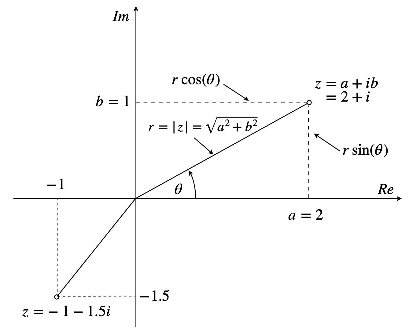
Figure 1. The Argand diagram showing two complex numbers in the form \(z = a + ib\), \(r\) is the modulus of the complex number \(z\) and \(\theta\) the argument measured anticlockwise from the real axis.
The Argand diagram is not like a normal graph in which a function such as \(y = x^3\) is plotted, because the value of \(y\) on the graph normally shows how large the function is at a given value of \(x\). The Argand diagram shows one point in the real and imaginary plane for each complex number so is more like a map that locates a place with latitude or longitude.
Performing algebra with complex numbers is no more difficult than with ‘normal’ numbers, because the prime rule of algebra still applies:
\(\qquad\qquad\)’Whatever I do to one side of an equation I do to the other side’
The normal rules for addition and multiplication apply but with the additional rule that additions and subtractions are kept separate for the real and imaginary parts, as is done for components of vectors. A complex number can be divided in the usual way by a real number. Dividing by a complex number has the additional step that the top and bottom of the expression are first multiplied by the complex conjugate of the denominator. This is explained below. Although \(i\) is a complex number, \(i^2 = -1\) and is a real number:
The series formed from the first few powers of \(i\) has a repeating pattern of four terms,
1.1 Complex conjugate#
Complex numbers possess a new property compared to real numbers and this is the complex conjugate. If \(z = a + ib\) then the complex conjugate is defined as
where, by convention, an asterisk is added and every \(i\) is replaced with \(-i\); the result is that \(z^*z\) is always a real number;
In geometrical terms, forming the complex conjugate is equivalent to a reflection in the real axis because only the imaginary part is inverted.
In quantum mechanics, the wavefunction is often found to be a complex quantity and, therefore, the complex conjugate is always used to calculate expectation or average values such as \(\displaystyle \langle x \rangle = \int\psi_i^* x\psi_f dx\) and probabilities \(\displaystyle p = \int \psi^*\psi dx\) because only a mathematically real quantity is measured in an experiment, not an imaginary one.
The quantity \(z + z^*\) is always a real number equal to \(2Re(z)\) or \(2Re(z^*)\) which is the same. It is worth remembering the rules
In some textbooks and some scientific papers, formulae involving complex numbers are written in a form that does not include the complex conjugate but instead has the notation +c.c. at the end of the equation to indicate that the complex conjugate is to be added. This is primarily a method of increasing the readability of formulae. An electric field describing linearly polarized light could be written as
instead of
similarly
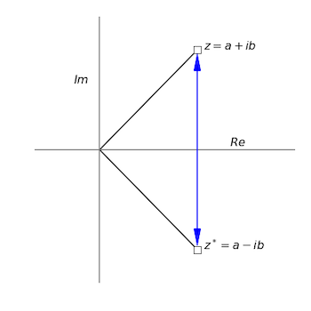
Figure 2. The complex number \(z\) and its complex conjugate \(z^*\).
1.2 Adding and subtracting complex numbers#
The real and imaginary parts are added separately as shown in Fig.3. This is very much like adding two vectors. Figure 3(Left) also illustrates the Triangle Inequality of complex numbers, i.e.
In figure 3 the absolute value of the complex number \(z_2\) is \(|z_2|\) of length \(r\). It can be seen that the green dotted line is less than the sum of one black and one red line, i.e. less than the sum of the magnitudes of the two complex numbers.
1.3 Multiplying and dividing complex numbers#
Multiplying complex numbers is straightforward using the normal rules of algebra but remembering to use \(i^2 = -1\) where necessary, e.g.,
Dividing numbers is a little more difficult. The rule to use is,
Always multiply the top and bottom of the whole expression by the complex conjugate of the denominator.
This is equivalent to multiplying by 1, and makes the denominator a real number. An example makes this clearer.
Figure 3. Left: Adding two complex numbers together to form \(z_1+z_2\) green dashed line. Right: Adding and subtracting \(z\) and its complex conjugate \(z^*\). The red arrow pointing down has the same length and angle as has \(z^*\) except that it starts at the end point of the line from the origin to \(z\) and ends at \(z+z^*\) The arrow going up is the reverse of that going down and leads to \(z-z^*\).
1.4 Modulus and Argument#
The second new property held by complex numbers is variously called the modulus, magnitude, absolute value, or norm of the complex number. This is calculated in a similar way to that of a vector and is the length of the complex number measured from the origin, Figs 1, 4.
The modulus \(r\) of the complex number \(z = a + ib\) is
It is variously written as
The square of a complex number is the square of the modulus;
and is always a positive number.
In figures 1 and 4 the line from the origin to the complex number is at an angle \(\theta\) given by
measured anticlockwise from the real axis. This angle \(\theta\) is variously called the argument, amplitude, polar angle, or phase of the complex number and is measured in radians, a full circle being \(2\pi\) radians. The use of the word ‘amplitude’ to mean an angle is very confusing, and should probably be avoided.
The location of any complex number is \((a,\; b)\) in Cartesian type coordinates, or alternatively, in polar type coordinates is \((r,\; \theta )\). The complex number is then described as
This interpretation is also illustrated in figure 1 for a point \(z = a + ib\) where \(r\) is the distance of the point from the origin. The distance along the real axis is \(a = r \cos(\theta)\) and along the imaginary axis, \(b = r \sin(\theta)\). Equating the real and imaginary parts gives
For example, if the complex number is \(z = i\), it has a real part that is \(0\) and an imaginary part of \(1\), and is represented by a point \((0, 1)\) which is on the imaginary axis. Its modulus is \(1\) and its argument (angle/phase) \(\pi/2\). If the number is \(z = -1 - i\) then the point is found at \((-1, -1)\) on the Argand diagram. Its argument is \(-5\pi/4\) (225\(^\mathrm{o}\)) and its modulus \(\sqrt{(-1 - i)(-1 + i)} = \sqrt{2}\).
1.5 Summary#
If \(a\) and \(b\) are real numbers, then the complex number is
\(\qquad\) \(z = a + ib = r\left(\cos(\theta) + i \sin(\theta)\right)\)
\(\qquad\) \(a = Re(z)\) is the real part of \(z\)
\(\qquad\) \(b = Im(z)\) is the imaginary part of \(z\)
\(\qquad\) \(r =|z|= \sqrt{z^*z}=\sqrt{a^2+b^2}\) is the modulus of \(z\), or absolute value, magnitude or norm.
\(\qquad\) \(\displaystyle \theta = \tan^{-1}\left(\frac{b}{a}\right)= \tan^{-1}\left( \frac{Im(z)}{Re(z)} \right)\) is the argument of \(z\), also called the polar angle or phase.
\(\qquad\) \(z^* = a - ib = r\left(\cos(\theta) - i \sin(\theta)\right)\) is the complex conjugate of \(z\).
\(\qquad\) \(zz^* = | z |^2 = | z^* |^2\) is the absolute value squared is always a positive real number.
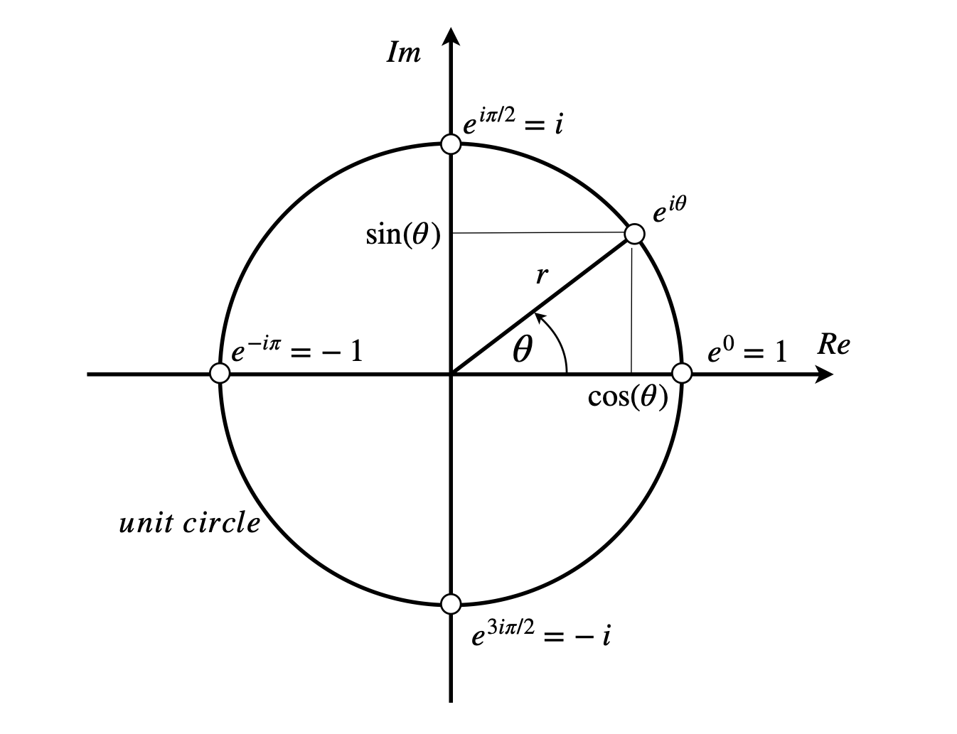
Figure 4. As the angle (argument) \(\theta\) varies anticlockwise from \(0\to 2\pi\), the complex number changes from \(1 \to i\) to \(-1\) to \(-i\) according to Euler’s theorem, equation 19. A unit circle has radius of \(1\).
2 Using Python and Sympy#
When using a computer language the complex number \(a+ib\) is not usually written in the mathematical way. In Python \(\mathtt{1J}\) or \(\mathtt{1j}\) is used instead of \(i\), thus \(\mathtt{3*1j}\) is permissible, however, so is \(\mathtt{3j}\) or \(\mathtt{5J}\). The parts of a complex number can be extracted by using the \(\mathtt{re()}\) and \(\mathtt{im()}\) functions. An alternative is to use \(\mathtt{z.real,\; z.imag}\) or \(\mathtt{z.conjugate()}\) (notice brackets) as shown below. In Sympy \(\mathtt{I}\) is used to represent \(i\), so care has to be taken not to use this as a variable or constant.
z0 = 3 + 5j
print(re(z0), im(z0) )
print( z0.real, z0.imag, z0.conjugate() )
3.00000000000000 5.00000000000000
3.0 5.0 (3-5j)
z1 = 6 - 4*1J
print(z0*z1,z0/z1)
(38+18j) (-0.03846153846153843+0.8076923076923077j)
In Sympy, however, \(\mathtt{I}\) is used to represent \(i\) but care has also to be taken in defining terms, for example
x = symbols('x',real=True)     #  Tell Sympy that x is not complex
exp(I*x).expand()              # try to expand e^ix as sine and cosine

which is not very helpful, instead \(x\) has to be defined as well as the \(\mathtt{expand( \cdots )}\) instruction being told that the expression is complex.
exp(I*x).expand(complex=True)

f = (3+5*I)/(1-2*I)
f.expand( complex = True )