
Solutions Q31 - 48
Contents
Solutions Q31 - 48#
# import all python add-ons etc that will be needed later on
%matplotlib inline
import numpy as np
import matplotlib.pyplot as plt
from sympy import *
init_printing()                      # allows printing of SymPy results in typeset maths format
plt.rcParams.update({'font.size': 16})  # set font size for plots
Q31 answer#
The three curves are shown in the polar plot below have \(a = 1\) and are shown in the order (a) to (c). The centre plot also shows, as a dashed line, the curve when the phase is ignored. The right-hand figure is plotted with \(n = 5\).
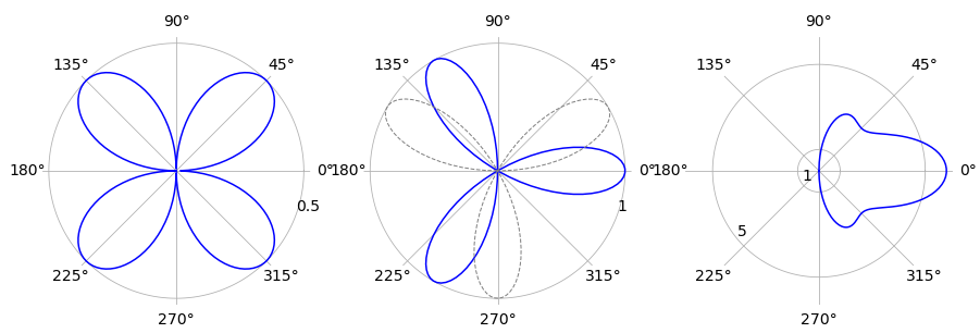
Figure 44 Polar plots; left curve (a), right (c).
(a) The angles when \(r=0\) are the solution to \(0 = a \cos(\theta)\sin(\theta)\) which are \(0\) and \(\pi/2\). The integration for one quarter of the area is therefore
and the total area is four times this. The integration can be evaluated by converting to exponentials. Using Sympy to do the integration is also straightforward,
theta, a = symbols('theta, a',positive = True)
eq = ((a*sin(theta)*cos(theta))**2)/2
integrate(eq,(theta,0,pi/2))

(b) This is tackled in the same way as (a) and the only difficulty is in finding the angles to use as integration limits. The equation to do this is \(0 = a \sin(3\theta + \pi/3)\) giving angles as \(k\pi/9\) where \(k\) can be one of the integers \(\cdots -2,\, -1, \,1,\,2 \cdots\) but not zero. The limits can be seen by plotting the graph either in polar or Cartesian coordinates. The first loop with small angles to the horizontal axis, has a range \(-\pi/9 \to 2\pi/9\). The area of just this loop is
and the total area is three times this value. The same result is obtained if the phase \(\pi/3\) is ignored and the limits taken as \(0 \to \pi/3\) instead.
(c) The integration angles with \(n=5\) are \(\pm \pi/2\) and the integration produces \(13a^2\pi/2\) as the area. The similar calculation with different \(n\) values shows that the limits are unchanged if \(n\) is odd. The general calculation using Sympy is
theta, a, n  = symbols('theta, a, n', positive = True)
eq = (a*(n*cos(theta) + cos(n*theta)))**2/2
simplify(integrate(eq,(theta,-pi/2,pi/2)))
however, as the sine and cosine terms are always zero if \(n\) is a positive integer the equation simplifies to produce \(a^2\pi(n^2 + 1)/4\) as the area with \(n \gt 1\) and odd. When \(n = 1\) the area is that of a circle \(\pi a^2\) and can be obtained from the integration result by using l’Hopital’s rule to obtain the limit since the denominator is zero when \(n = 1\). The calculation is a straightforward but long one.
Q32 answer#
In the plot, curve(a) is on the left and the right-hand figure curve (b) has \(n = 5\) and both are plotted with \(a = 1\).
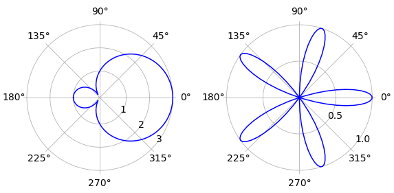
Figure 45. Polar plots, left curve (a). Note that some graphics applications will plot the small loop in (a) inside the larger one.
(a) The limits to the integration are multiples of \(\pm 2\pi n/3\). By plotting we find that the outer curve, starting and ending at the pole has limits \(-2\pi/3 \to +2\pi/3\) and the inner loop from $+2\pi/3 \to +4\pi/3. The outer area is therefore
The inner loop has area
making the area excluding the loop \(a^2(3\sqrt{3} + \pi)\). The inner loop calculation using Sympy is
theta, a, n  = symbols('theta, a, n', positive = True)
eq = a**2*(2*cos(theta) + 1)**2/2
simplify(integrate(eq,(theta,2*pi/3,4*pi/3)))

(b) If \(n=1\),the equation is that of a circle of radius \(a/2\) with its centre at \(r = 1/2\) and \( \theta= 0\). The difference in area to that of a circle of radius \(a\) is therefore \(3\pi a^2/4\). The plot shows the curve produced when \(n = 5\). The radius vector is zero at angles \(\pm k \pi/10\) where \(k\) is an integer. The limits \(\pm \pi/10\) cover the loop on the horizontal axis. By symmetry, the area of all five loops is then just five times this value. Using Sympy
theta, a  = symbols('theta, a', positive = True)
n = 5
eq = n*a**2*(cos(n*theta) )**2/2
simplify(integrate(eq,(theta,-pi/(2*n),pi/(2*n))))

which is clearly going to produce \(3\pi a^2/4\) as the area between the five-leaved figure and the circle. If the calculation is repeated with different integer n values the same result is obtained when the limits are changed as appropriate to \(\pm \pi/2n\). It does not look as if only one quarter of the area is filled by the loops in the curve, particularly if curves with \(n = 200\) or other large numbers are potted. Even stranger is that in the limit \(n \to \infty\) it appears that the unfilled area is still the same; an infinite number of loops is present but each of infinitesimal thickness and they do not fill all the space.
Q33 answer#
If OA = \(\cosh(\theta)\) let the angle BOA be \(\theta\), then by definition \(\tanh(\theta) = \sinh(\theta)/\cosh(\theta)\)
and in a right-angled triangle, because \(\tanh\) = opposite / adjacent, AB = \(\sinh(\theta)\). Generalizing, because A can be at any distance along the axis, gives \(x = \cosh(\theta)\) and as the equation of the curve is \(x^2 - y^2 =1\) therefore \(y^2 = x^2 -1 = \cosh^2(\theta)-1\). From the definitions of hyperbolic functions (Chapter 1.5.5) \(\cosh^2(\theta) - \sinh^2(\theta) = 1\). This can easily be proved because by definition,
Substituting for \(x\) gives \(y^2 = \cosh^2(\theta) - 1 = \sinh^2(\theta)\) and therefore the equation of the curve \(x^2 - y^2 = 1\) is also \(\cosh^2(\theta) - \sinh^2(\theta) = 1\).
The area QAB is the area of the triangle less that of the integral of the curve from Q to A. First the area of the triangle OAB is half base \(\times\) height which is \(\sinh(\theta)\cosh(\theta)/2\). Using \(x=\cosh(\theta) \) and \( dx=\sinh(\theta) d\theta\), the integral is
Integration is easier by converting the hyperbolic functions into their exponential form,
The area QAB is therefore
which after changing to exponential form produces the area QAB = \(\theta/2\).
Q34 answer#
First plot the function using polar coordinates with a \(\mathtt{plt.polar(theta, r(theta) )}\) type of plot. To help calculate the limits plot \(1 + 2\sin(x) = 0\) in Cartesian coordinates, shown below on the right. A root of this equation occurs at \(\theta = -\pi/6\) and at \(\theta = -5\pi/6\) and then at \(\pm 2\pi\) intervals or \(\theta=-\pi/6+2\pi,\theta=-5\pi/6+2\pi\) etc. as shown in the figure.
By plotting only between limits, it is found that the negative areas on the right-hand plot correspond to the smaller loop in the polar plot. Note that some graphics packages may put the smaller loop inside the larger one.
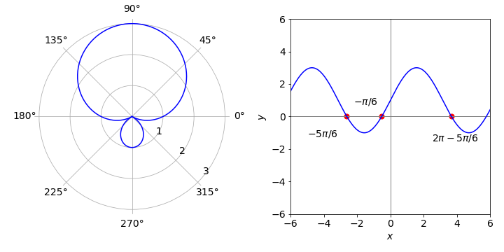
Figure 46. Polar coordinate plot. The zeros are also shown on the right hand plot. Right: Normal or Cartesian plot.
(b) The total area enclosed by the curve is \(\displaystyle \frac{1}{2}\int_0^{2\pi} (1+2\sin(\theta))^2 d\theta=3\pi\)
(c) The inner curve has an area with limits \(\theta = -5\pi/6 \to θ = -\pi/6\) and as \(\sin(\pi/6) = \sin(5\pi/6) = 1/2\) and \(\cos(\pi /6) = -\cos(5\pi/6)=\sqrt{3}/2\), the integral has the value \(\pi-3\sqrt{3/4}\).
Q35 answer#
The integration is \(\displaystyle A=\frac{a^2}{2}\int_a^b(1+\cos(\theta))^2 d \theta\)
where the limits are defined by which part of the figure is being calculated. Because the cardioid is symmetrical, limits of \(\pi/2 \le \theta \le \pi\) can be used for the backward going signal and the result doubled. Similarly the total area is twice that with \(0 \le \theta \le \pi\) this is
The backward projecting signal is calculated from the same integral but with limits \(\pi/2 \to \pi\) and has the value \(a^2(3\pi -8)/4\). The ratio is \((3\pi-8)/(6\pi)\) which is \(\approx 0.076\) so that only \(7.6\) % of the signal is lost.
Q36 answer#
(a) The function is \(f (t) = a\) which is a constant and by definition
Substituting gives \(L(a)\equiv F(s)=a/s\).
(b) Let \(L(ae^{at})=\int_0^\infty e^{at-st}dt= 1/(s-a)\) provided \(s \ne a\)
(c) \(L(t) =\int_0^\infty te^{-st}dt=1/s^2\)
(d)\( L(f(at))=\int_0^\infty f(at)e^{-st}dt\). To solve this let \(at=v\) then
and the last step is made by comparison with the definition of \(F(s)\) in the question.
(e)Integrating by parts with \(\displaystyle dv=\frac{df(t)}{dt}\) and \(u=e^{-st}\) then
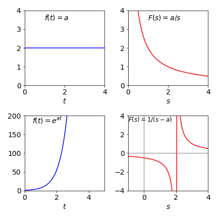
Figure 47. Two functions (left) and their Laplace transforms (right)
Q37 answer#
The area is the integral \(\displaystyle \int_{x_0}^\infty x^2e^{-\alpha x^2}dx\) and should be identified as one of the special integrals that are best looked up of solved using Sympy. It is not simple to do this by hand.
x, x0, alpha  = symbols('x, x0, alpha', positive = True)
eq = x**2*exp(-alpha*x**2)
simplify(integrate(eq,(x,x0,oo)))
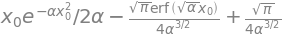
The error function is defined as the integral
and ranges from \(0\to 1\). Notice that the variable \(x\) is in the limit of the integration. The error function represents the area under the Gaussian, or bell shaped, normal distribution curve, and is therefore frequently met in statistics.
Q38 answer#
Integrating directly produces the general equation;
x, alpha, n  = symbols('x, alpha, n', positive = True)
eq = x**n*exp(-alpha*x**2)
simplify(integrate(eq,(x,-oo,oo))  )

where \(\Gamma(..)\) is the gamma function. See chapter 1.7 for a graph. For integer \(n\) the gamma function produces factorials as \(\Gamma(n+1)=n!\). Because of the \((1+(-1)^n)\) term the integral is zero for odd values of \(n\). This is expected since when \(n\) is odd then so is \(x^ne^{-\alpha x}\) and the area under the curve for an odd function, provided the limits are symmetrical, is always zero.
The even \(n\) integrals can be easily simplified because the gamma function has the property
for integer \(m\). The double factorial has the form \(n!!=n(n-2)(n-4)\cdots \). The first few terms are \(\Gamma(1/2)=\sqrt{\pi},\; \Gamma(3/2)= \sqrt{\pi}/2,\; \Gamma(3/2)=3\sqrt{\pi}/4\)
Q39 answer#
‘By inspection’ means ‘evaluate without doing any numerical calculations’, thus work out the answer logically. Because \(e^{-x^2} =e^{-(-x)^2}\), all the parts of the wave functions are even. The terms \(x^n\) where \(n\) is odd, are ‘odd’ functions and vice versa, therefore the total wavefunction with even quantum numbers are ‘even’ functions, and those with odd quantum numbers are ‘odd’ functions. If you are still not convinced draw the wavefunctions; two of them \(\psi_2\) and \(\psi_3\), are shown using values for the vibration in CO with \(x\) from \(-30 \to 30\) pm. The vertical scales are arbitrary.
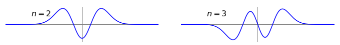
Figure 48. Harmonic oscillator vibrational wavefunctions with parameters for CO; \(n = 2\) is an even function, \(n = 3\) an odd one.
Q40 answer#
(a, b) The wavefunctions are
and \( N_0 = (\alpha/\pi)^{1/4},\; \alpha = \sqrt{k\mu/\hbar}\) where \(k\) is the force constant and \(\mu\) reduced mass. If the wavefunctions are orthogonal \(\displaystyle \int_{-\infty}^\infty \psi_i^*\psi_j dx=0\).
The product of the wavefunctions is
and as an integral of this form has ‘odd’ character and the limits are symmetrical about zero it is expected to be zero. To prove this substitute \(u=x^2,\, du=2xdx\), which makes both limits \(\infty\) and if the limits are the same any integral must be zero; \(Q\sim \int_\infty^\infty e^{-\alpha u}du=0\).
We therefore conclude that \(\psi_1\) and \(\psi_2\) are orthogonal.
(c) To check the normalization of \(\psi\) use
This cannot be integrated to an algebraic expression but instead involves the eror function which itself is an integral. All integrals of the form \(\displaystyle x^ne^{-\alpha x^2}dx\) when \(n\) is even involve the error function. The general form is
where \(c\) is the integration constant. Using Sympy gives this answer.
x, alpha, n  = symbols('x, alpha, n', positive = True)
eq = exp(-alpha*x**2)
simplify(integrate(eq,x ))

Using the properties of the error function, \(\mathrm{erf} (0) = 0,\; \mathrm{erf} (\pm\infty) = \pm 1\) the integral with limits is \(\sqrt{\pi /\alpha}\) and therefore \(\displaystyle Q_0= \sqrt{\frac{\alpha}{\pi}}\sqrt{\frac{\pi}{\alpha}}=1\) and the wavefunction is normalised.
Q41 answer#
Substituting gives \(\displaystyle e^{t\tau}=k_1N\int_0^\infty e^{r(t-\tau)}e^{-k_2t}dt=k_1Ne^{rt}\int_0^\infty e^{-(r+k_2)t}dt\)
simplifying and integrating gives \(\displaystyle 1=\frac{k_1N}{r+k_2}e^{-(r+k_2)t}\bigg|_0^\infty =\frac{k_1N}{r+k_2}\) producing \(r=k_1N-k_2\).
Q42 answer#
(a) Orthogonality means that the integrals of the products of two wavefunctions have the behaviour
which means that the integral is \(0\) unless \(j = k\). The delta function has the property if \(j \ne k,\; \delta_{j,k} = 0\) ortherwise \(\delta_{j,k} = 1\).
If the wavefunctions are normalized when \(j = k\), this integral is \(1\) as has been implicitly assumed.
If the wavefunctions are eigenstates of the molecule, i.e. solve the Schroedinger equation, they are always orthogonal to one another but may not necessarily be normalized. Normalizing wavefunctions is something that we can easily do by making \(\int \psi_k^*k\psi_k dx = 1\) by multiplying \(\psi\) by a constant.
(b) The integral has three terms, two wavefunctions and the transition dipole. The integral must not be identically zero if the transition is allowed, if the integral is not to be identically zero the product \(\psi_i^*\psi_f\) must have the same symmetry, i.e. ‘odd’ as the dipole \(\mu x\) making an ‘even’ symmetry function overall inside the integral. If wavefunctions in states \(f\) and \(i\) were the same, either both even or both odd, then \(\psi_i^*\psi_f\) would be even and when multiplied by \(\mu x\) would become ‘odd’ overall and the integral zero. More precisely if the symmetry species of the two wavefunctions were the same, their direct product would belong to the totally symmetric representation of the molecule’s point group.
In this question because \(\mu x\) is always odd, it cannot belong to a totally symmetric representation. The integral eqn. 20 will be identically zero and the transition forbidden. In two photon transitions that can occur with high laser intensities, the transition dipole moment \(\mu x\) would be squared inside the integral and therefore be an even quantity making such transitions allowed.
Q43 answer#
(a) Substituting for \(\mu x\) into equation 20 and rearranging without doing any calculation produces
The last line is repeated but in the bra-ket form which is clearer.
Different wavefunctions are orthogonal because they are in the same electronic state (in this case the ground state) which means that
Studying the equations for the wavefunctions leads also to this conclusion,
The molecule must therefore have a permanent dipole if a vibrational transition is to occur, provided that the derivative \((d\mu_0/dx)_0\) is not zero. However, the charge distribution in the molecule ensures it will never be exactly zero if a dipole exists. If this derivative is small you would naturally expect that the transition has little intensity.
(b) The second integral is only finite when the vibrational quantum state is within one unit of the initial one or \(f = i \pm 1\). The selection rule for vibrational transitions is usually written as \(\Delta n=\pm 1\). Consider the \(n = 0 \to n = 1\) transition, using equations from question 39,
and the complex conjugates are not needed since the wavefunctions are real. This integral is evaluated with Sympy in questions 37 and 38, and its value is
where \(N_0=(\alpha/\pi)^{1/4}\) was given in Q 40. This equation is multiplied by \(d\mu/dx\) which is often unknown, but is not zero, so that the transition moment is
and has the dimension of length. As an aside, a photon contains one unit of angular momentum, which is destroyed on absorption and transferred to the molecule so that overall there is no momentum change. A vibrational change does not involve any angular momentum: the motion is linear so it follows that in a vibrational transition rotational motion of the molecule is changed by absorption, i.e a vibrational transition is also accompanied by a change in rotational energy also.
Exercise:(a) calculate \(Q\) for the \(1\to 2\) transition and (b) use Hermite polynomials for the general \(n\to m \) transition.
Q44 answer#
(a) Starting with \(\displaystyle J_{flux}=-D\left( \frac{zFc}{RT}\frac{dV}{dx}+\frac{dc}{dx} \right)\),
where \(D\) has units of \(\mathrm{m^2\,s^{-1}}\), \(c\) mole m\(^{-3}\), \(F\) Coulomb/mole, \(V\) volts (J/C) , \(x\) metres, \(T\) temperature (K), \(R\) the gas constant \(\mathrm{J\,K^{-1}\,mole^{-1}}\), and \(z\) is a number. The equation has units
When multiplied by \(zF\) the units become \(\displaystyle I\equiv \mathrm{\frac{C\, mole}{m^2\,s\,mole}=\frac{A}{m^2} }\) because an ampere is a Coulomb/second.
(b) Starting with equation 23 and differentiating, and remembering that \(V\) and \(c\) are functions of \(x\), gives
and multiplying this result by the constants \(-zDF\) should make this expression equal to \(Ie^{zFV/RT}\) and then eliminating the exponentials from both sides gives equation 22.
(c) Integrating the right-hand side of equation 23 is easy because it is already a derivative;
and the concentrations are \(c_a, \,c_b\) and voltages \(V_a,\, V_b\) depend upon where they are measured,i.e. position \(a\) or \(b\). Integrating the left-hand side seems to be straightforward because it appears not to depend on \(x\), but recall that \(V\) depends on \(x\) and therefore it is necessary to know what this dependence is; luckily it is known and is \(V = Ex\). The integration is still simple however,
where the substitutions \(V_b=Eb,\, V_a=Ea\) have been made. Combining both sides of the equation gives
which can be simplified by writing \(\Delta V = V_b - V_a\). As described in the question the electric field in the pre-factor is proportional to the voltage difference and this can be changed to \(E = \alpha \Delta V\) giving
This is the Goldman-Hodgkin-Katz equation.
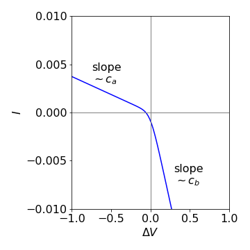
Figure 49 Current-voltage curve of the Goldman-Hodgkin-Katz equation. \(z=1,\,T= 300 \mathrm{K},\,c_b =10^{-4} \mathrm{dm^3\, mol^{-1 }},\,c_a=c_b/10 \).
(d) In the limit of large \(+\Delta V\) the exponential terms in equation 99 are very large, much greater than unity or \(c_a\) so these terms cancel out leaving
which is equivalent to Ohm’s law; current is proportional to voltage with the proportionality here being the reciprocal of the resistance.
At large negative potential difference, the exponential terms tend to zero giving
The slope of current vs voltage is now proportional to \(c_a\) compared to the limit at large positive potential difference, where the slope was proportional to \(c_b\).
(e) A graph of the current-voltage curve is shown in Figure 49 with \(z=1,\,T= 300 \mathrm{K},\,c_b =10^{-4} \mathrm{dm^3\, mol^{-1 }}\), \(c_a=c_b/10 \) and the constant \(\alpha = 10^6\) is used only to scale the current for plotting. \(F = 96487\, \mathrm{C\,mol^{-1}}\).
Notes: The flux is produced by supposing that there is a force \(f_v\) that is proportional to the velocity of the molecules or ions \(F_v = -fv\) and opposes their motion, hence the negative sign. The constant of proportionality \(f\) is the coefficient of friction. The average flux is the concentration \(c(x)\) at some point \(x\) in the solution multiplied by the average velocity of the molecules,
The imposed or external force causes a concentration gradient and if equilibrium is established then the flux due to the force will balance that due to the concentration gradient; the latter is by Fick’s Law
The equation of balance is
and the concentration can be given by a Boltzmann distribution with energy controlled by the external force \(\displaystyle c(x) = c_0e^{F_v x /k_BT}\). Differentiating and simplifying gives \(\displaystyle \frac{1}{f}-\frac{D}{k_BT}=0\) which is the expression first derived by Einstein
If the flux is not balanced,
The force is \(F_v = dV/dx\) when a voltage is applied.
Exercise: Rationalize the size of the current when the temperature is very small and very large, i.e. tending to zero or infinity.Recall that the diffusion coefficient depends on temperature as \(D = k_BT/f\) where \(f\) is the constant friction imposed by the solvent in which the ion or molecule is diffusing. Consider separate cases when the voltage is positive and when negative.
Q45 answer#
(a) The ions are both singly charged so that \(q_1\) and \(q_2\) are \(+e\) and \(-e\) respectively where \(e\) is the electronic charge. The ions move from infinity to \(r\) , so the work done is the integral from infinity to \(r_0\),
The constants are \(e = 1.62 \cdot 10^{-19}\;\) C, the permittivity of free space \(\epsilon_0 = 8.854 \cdot 10^{-12}\mathrm{ C^2 \,J^{-1}\, m^{-1} (\equiv F\,m^{-1})}\) and the dielectric constant (relative permittivity) of water \(\epsilon = 80\). Substituting for \(r_0\) the energy is \(E = -2.95 \cdot 10^{-21}\) J/molecule which at \(300\) K is comparable to thermal energy \(k_BT = 4.14 \cdot 10^{-21}\) J. The negative value of the energy means that the force is attractive as expected for oppositely charged ions.
(b) For the non-polar solvent \(\epsilon=2\), the energy is 40 times greater, which is the ratio of dielectric constants, and is \(-118 \cdot 10^{-21}\) J.
(c) This energy is obviously greater because the dielectric constant is smaller and the ions are attracted to one another more strongly at any distance than at the same distance in water. A low dielectric medium does not attenuate an ion’s electric field as much as a higher one would. This means that in water the attractive energy is comparable to thermal energy, which can therefore disrupt their interaction, and the ions can more or less move freely. In a solvent such as a liquid hydrocarbon, hexane, or benzene perhaps, which has a low dielectric constant, the attractive energy is so high compared to thermal energy at room temperature that the ions will largely remain in each other’s vicinity, i.e. as an ion-pair. A general observation is that salts do not dissolve in hydrocarbons.
Q46 answer#
(a) Using the information in the question, the work done, or equivalently, the energy needed, is
This equation was first derived by Born.
(b) Now move the ion ( radius \(r=0.2\) nm) into the membrane. The energy needed is the difference the energy the ion has in water vs that in the membrane which is
and is positive as the ion is more stable in water because its dielectric constant is larger. The energy change is \(\approx 68\) times thermal energy at \(300 \mathrm{K} \;,k_BT = 4.14 \cdot 10^{-21}\) J, so it is very unlikely to happen spontaneously and shows how unfavourable it is to move an ion into a lipid membrane from water.
(c) The rate constant can be estimated using Arrhenius’ equation and even if the pre-exponential factor is \(10^{12}\, \mathrm{s^{-1}}\), the rate is still \(\approx 10^{-18}\mathrm{\, s^{-1}}\), which is staggeringly small and equivalent to occurring once in approximately \(10^{11}\) years. This is why nature has to use membrane bound proteins to pass ions through membranes rather than relying on direct diffusion.
Q47 answer#
(a) The equation for \(P(u)\) has the form met before which is, \(x^2e^{-\alpha x^2}\). Either integrate this expression or substitute for \(\alpha\) and multiply by the constants before the \(u^2\) term, or use Sympy to recalculate the whole expression; \(\alpha=m/(2k_BT)\)
The equation for normalization is \(\displaystyle \int_0^\infty p(u)du\)
u, u0, alpha = symbols('u, u0, alpha',positive =True)
Pu= 4*pi*(alpha/pi)**(3/2)*u**2 *exp(-alpha*u**2)
integrate(Pu,(u,0,oo))

(b) The initial speed is now \(u_0\) not zero, therefore the calculation is essentially the same as in part (a) but with limits \(u_0,\,\infty\), gives the probability as
simplify(integrate(Pu,(u,u0,oo)) )
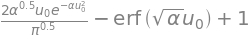
which when \(\alpha\) is substituted for gives
which is the cumulative probability that molecules have a speed \(\ge u_0\). When the speed is zero the error function is also zero. Therefore, the cumulative probability of having a speed \(\ge 0\) is \(1\), which it must be, and this means that the speed probability distribution is normalized, as has already been proved. You can appreciate this also by observing how the curves change when the temperature is lowered. The curves become narrower and higher and peak at a lower speed. This occurs because the area is always constant, in this case at unity because the probability is normalized.
(c) The probability that the molecules have a speed greater that \(350 \,\mathrm{m \,s^{-1}}\) is the area of the distribution above this speed and is \(prob(350, T, m)\). Substituting values produces the following table for the chance of having a speed greater than \(350\, \mathrm{m \,s^{-1}}\) at different temperatures. The graph shows the \(350\, \mathrm{m \,s^{-1}}\) probability curve vs temperature.
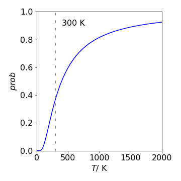
Figure 50. The probability (fraction) of SO\(_2\) molecules that have a speed greater than \(350 \,\mathrm{m \,s^{-1}}\) vs temperature.
The values in the graph and table make sense because the higher is the temperature the more energy the molecules have and the faster they move, therefore more of them must have a speed greater than \(350\, \mathrm{m \,s^{-1}}\). See Fig. 3.48.
(d) The energy distribution is obtained from equation 24 by substituting \(E = (1/2)mu^2\) to give
which when simplified is independent of the mass as may be anticipated.
The fraction of molecules with energy above \(k_BT\) is the fraction above this energy which is \(\displaystyle \int_{k_BT}^\infty P(E)dE\). Using Sympy gives
E, kBT, m = symbols('E, kBT, m',positive = True)
PE= 4*pi*sqrt((m/(2*pi*kBT))**3)*(2*E/m)*exp(-E/(kBT))/sqrt(2*m*E)
simplify(integrate(PE,(E,kBT,oo) ) )

hence the integral is
which means that for any temperature \(57.2\)% of all molecules have energy above \(k_BT\).
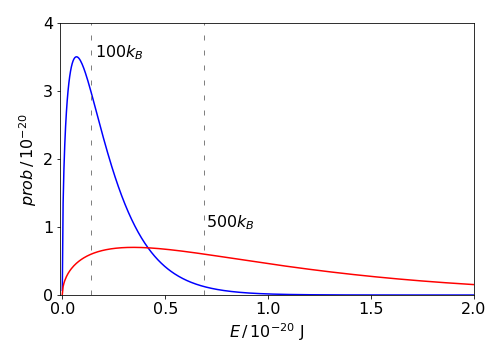
Figure 51. The energy probability distribution for molecules at 100 (blue) and 500 K (red) together with the energies \(k_BT\) which divide the areas so that 57% of the molecules have more than this energy at each temperature. The energy is in joules per molecule.
Q48 answer#
(a) With an escape velocity of \(2350 \,\mathrm{ms^{-1}}\) and a temperature of \(380\) K the fraction \(0.0653\) of He atoms and \(6.2 \cdot 10^{-11}\) of N\(_2\) molecules escape from the moon’s gravity. Once a molecule has escaped, the remainder will re-equilibrate to a new temperature because a little of the initial energy has been lost. As bimolecular collisions between molecules are very rare there being no atmosphere, re-equilibration should be an exceptionally slow process but could occur instead via collisions with the moon’s surface. Nevertheless, on the geological time scale of millions of years, re-equilibration would be rapid and so all the molecules would escape, although for N\(_2\) this will take far longer to do so than for He.
(b) The similar calculation for the earth produces fractions that escape as \(2.05 \cdot 10^{-9}\) for He and \(1.6 \cdot 10^{-65}\) for N\(_2\) assuming that the temperature is \(1400\) K at \(1000\) km. Both these fractions are small and the rate of escape by speed alone will depend on the re-equilibration rate due to collisions causing a steady state concentration gradient to be produced. The amount of He lost is small but on a geological time scale not much would remain if it were not continuously generated by radioactive decay in some rocks; the amount in the atmosphere is therefore a balance of loss and gain. The amount of nitrogen lost is so infinitesimal that even on a geological timescales of millions of years, it will not be lost to space and less so when multiplied by the fraction of all molecules present at that altitude as calculated in (c). For example, the atmosphere weighs \(\approx 5 \cdot 10^{18}\) kg (Chapter 1.12) and contains \(\approx 1.5 \cdots 10^{20}\) mol N\(_2\), and \(10^{-65}\) of this is still utterly minute.
(c) The potential energy of a molecule at altitude \(h\) is \(mgh\) so that the fraction is
where \(g\) is the acceleration due to gravity; on earth, this is \(9.81\, \mathrm{m \,s^{-2}}\). Also on earth at \(100\) km and \(1400\) K, the fraction of He is \(0.71\) and \(0.094\) for N\(_2\). (This assumes that all the gas is at \(1400\) K whereas much of the atmosphere is far cooler, \(300\) K or less, therefore these numbers are greater than the true amounts.
At \(300\) K the fraction of He is \(\approx 0.2,\, \mathrm{N_2} \approx 1.6 \cdot 10^{-5}\). The He is so light that gravity has a small effect on it and a significant fraction is present at high altitudes whatever the temperature and so there must be a nearly constant concentration with altitude unless significant amounts are lost into space. The temperature is significantly higher (\(1400\) K) at \(100\) km, than at the surface, making it more likely that the escape velocity can be exceeded. However, only \(\approx 2 \cdot 10^{-9}\times f\) of all He atoms will exceed the escape velocity at this temperature where \(f\) is the fraction between \(0.7\) and \(0.2\) present at \(100\) km, and although this is small, over geological time, it will deplete all the He in the atmosphere. Without knowing the rates of He production and loss to space or into the oceans or elsewhere, unfortunately, little more can be concluded about the amount in the atmosphere.
At high altitudes, molecules and atoms can be ionized by UV and shorter wavelength radiation and by charged particles from the sun and it seems likely that the earth’s magnetic field will constrain most of these ions and return them to the poles where recombination can occur to produce neutral species. Whether this is a significant process is left for you to investigate.
On the moon, the acceleration due to gravity is \(1.62\,\mathrm{ m \,s^{-2}}\), which is much reduced from that on earth by the ratio of their respective masses and radii squared. The fraction of He at \(100\) km is \(0.75\), and it is \(0.24\) at \(500\) km so we expect these gases to escape either when ionized, because the moon has no strong magnetic field to deflect charges particles from the sun, or as neutral species.