8 Perturbation Theory#

# import all python add-ons etc that will be needed later on
%matplotlib inline
import numpy as np
import matplotlib.pyplot as plt
from sympy import *
from scipy.integrate import quad
init_printing()                      # allows printing of SymPy results in typeset maths format
plt.rcParams.update({'font.size': 14})  # set font size for plots

8 Perturbations#

Solving the Schroedinger for the energy levels of a molecule, using a model such as a harmonic oscillator or rigid rotor, allows us to predict the spectrum. These spectral lines may, however, only be close to the experimental values not exactly matching them because of small unsuspected interactions. To investigate how to improve our model to better understand the data, changes to the potential energy are necessary. The harmonic oscillator, for example, has the Hamiltonian,

\[\displaystyle H^0=-\frac{\hbar^2}{2m}\frac{d^2}{dx^2}+\frac{k}{2}x^2\]

where the potential energy \(\displaystyle V(x)= kx^2/2\). We might try to improve on this, perhaps by adding cubic or quartic terms, such as \(ax^3 + bx^4\), to describe the effect of the bond stretching. Similarly, we might consider adding terms in \(J^4\) to the rigid rotor model to allow for centrifugal distortion during rotation. Alternatively, the harmonic potential model may be satisfactory, but the experiments report on the effects of small changes to the spectrum caused by external electric or magnetic fields. In this case, if the electric field \(E\) is along the x-axis a term \(E ex\) could be added to the Hamiltonian to allow for this. The use of perturbation theory allows for the incorporation of these and many other small potential energy terms to extend our knowledge a little into unfamiliar territory by using what is already known as a starting point.

Our aim is to be able to express the perturbed energy levels \(E_n\) in terms of the unperturbed energies \(E_n^0\) and their wavefunctions \(\psi _n^0\) both of which are assumed to be known from solving \(H^0\psi^0 = E^0\psi^0\).

8.1 Formal derivation.#

First, the formal derivation is presented in most of the important details and the rather simple results, equations (41) and (43), that describe the changes in energy and wavefunctions are produced. These equations are then applied to some examples. If you want to try the problems and are not interested in the derivation details, then these equations are the results you will need.

The Schroedinger equation whose solutions are known, is defined as,

\[\displaystyle H^0\psi_n^0 = E_n^0\psi_n^0 \qquad\tag{31}\]

The superscript 0 indicate that the wavefunctions and energies are known for every quantum number \(n\) = 0, 1, 2, \(\cdots\). Later on we use the notation \(\psi^{(2)}\) etc., explained further below, in which the brackets indicate the second derivative not the square. However when the supescript is zero we do not add brackets as it is unambiguous.

The wavefunctions form an orthonormal set so that

\[\displaystyle \int \psi^{0*}_n\psi_m^0 d\tau = \delta_{nm} \qquad\tag{32}\]

and formally the equation is solved by left multiplying equation (31) by a wavefunction and integrating. The result is

\[\displaystyle \int \psi^{0*}_nH^0\psi_m^0 d\tau =E_n^0\int \psi_n^{0*}\psi_m^0 d\tau = \delta_{nm}E_n^0 \qquad\tag{33}\]

where \(\delta_{nm}\) is the Kronecker delta function which is zero unless \(n = m\) when it is unity. (Note that \(n\) and \(m\) are both dummy indices labelling energy levels, it does not matter if they are exchanged; i.e. equation (31) could be labelled with \(m\)’s rather than \(n\)’s.)

An extra potential term is now added to the Hamiltonian operator, changing it from \(\displaystyle H^0=-\frac{\hbar^2}{2m}\frac{d^2}{dx^2}+V(x)\), whose solution is known to,

\[\displaystyle H=H^0+\lambda V\]

whose solution is sought. It is assumed that the potential term \(V \ll V_0\) produces only a small perturbation to the system. The parameter \(\lambda\) is a dimensionless coefficient that is allowed to vary from zero, which is no perturbation, to one, the full perturbation. It is not necessary to know what \(\lambda\) is; it is only as a way of reaching an answer. To make the calculation simpler, the energy levels \(E_n^0\) are always assumed to be non-degenerate. Degenerate levels can be dealt with in a similar manner; see Atkins & Friedmann (1997),

The perturbed Schroedinger equation is

\[\displaystyle H\varphi_n = E_n\varphi_n \quad \mathrm{ or } \quad \left(H^0 + \lambda V\right)=\varphi_n=E_n\varphi_n \qquad\tag{35}\]

where all the new wavefunctions \(\varphi_n\) and energies \(E_n\) are unknown so far. Both the wavefunction \(\varphi\) and energy are functions of the parameter \(\lambda\). Our aim is to be able to express the perturbed energy levels \(E_n\) in terms of the unperturbed energies \(E_n^0\) and their wavefunctions \(\psi_n^0\) both of which are already known. The assumption is now made that perturbed energies and wavefunctions can be expanded as Taylor series in \(\lambda\); see equation (15). This assumption is justified by the validity of the final result. Expanding \(E\) and \(\varphi\) gives

\[\displaystyle E_n = E_n\mid_{\lambda = 0} + \lambda \left[\frac{dE_n}{d\lambda} \right]_{\lambda = 0} +\frac{\lambda^2}{2!} \left[\frac{d^2E_n}{d\lambda^2} \right]_{\lambda = 0}+ \cdots \]

\[\displaystyle \varphi_n = \varphi_n\mid_{\lambda = 0} + \lambda \left[\frac{d\varphi_n}{d\lambda} \right]_{\lambda = 0} +\frac{\lambda^2}{2!} \left[\frac{d^2\varphi_n}{d\lambda^2} \right]_{\lambda = 0}+ \cdots \]

A new notation is now introduced to make the equations simpler to read,

\[\displaystyle E_n^{(j)} = \left[ \frac{1}{j!} \frac{d^jE_n}{d\lambda^j} \right]_{\lambda=0} \qquad \varphi _n^{(j)} = \left[ \frac{1}{j!} \frac{d^j\varphi_n}{d\lambda^j} \right]_{\lambda=0} \]

therefore

\[\displaystyle E_n = E_n^0 + \lambda E_n^{(1)} + \lambda ^2E_n^{(2)} + \cdots \qquad\tag{36} \]

\[\displaystyle \varphi_n = \psi_n^0 + \lambda \varphi_n^{(1)} + \lambda^2\varphi_n^{(2)} + \cdots \qquad\tag{37}\]

Notice that \(E(0) \equiv E^0\) is the unperturbed energy and \(\varphi(0) \equiv \psi^0\) the unperturbed wave- function. Next, \(E\) and \(\varphi\) are substituted into the perturbed Schroedinger equation (35) and an apparently very complicated equation results;

\[\begin{split}\displaystyle \begin{align}\left(H^0+\lambda V\right)&\left(\psi_n^0 + \lambda \varphi_n^{(1)} + \lambda^2\varphi_n^{(2)} + \cdots\right)\\&=\left(E_n^0 + \lambda E_n^{(1)} + \lambda ^2E_n^{(2)} + \cdots\right)\left(\psi_n^0 + \lambda \varphi_n^{(1)} + \lambda^2\varphi_n^{(2)} + \cdots\right) \qquad\qquad\qquad\text{(38a)}\end{align}\end{split}\]

However, grouping terms with similar powers of \(\lambda\) allows equation (38) to be rearranged in a far clearer way;

\[\begin{split}\displaystyle \begin{align}&(H^0+E_n^0)\psi_n^0 +\\ &\lambda \left[(V-E_n^{(1)})\psi_n^0 + (H^0-E_n^{(0)})\varphi_n^{(1)} \right] + \\ &\lambda^2 \left[(V-E_n^{(1)})\varphi_n^{(1)} + (H^0-E_n^{(0)})\varphi_n^{(2)}\right ] + \lambda^3\left[\cdots\right]+\cdots =0\end{align} \end{split}\]

The zeroth-order term is the initial unperturbed equation. Technically it is multiplied by \(\lambda^0\) (\(\lambda\) to power 0) but as this is \(1\), it is not written explicitly. When each term multiplied by \(\lambda\) is added together the sum is zero and thus each term in square brackets is itself zero.

First order correction to the energy#

To obtain the first-order correction to the energy it is assumed that \(\lambda^2\) is smaller than \(\lambda\) and similarly for higher powers and therefore these can be ignored. The first-order energy correction is obtained by extracting just the terms in \(\lambda\) and is

\[\displaystyle \left(V-E_n^{(1)}\right)\psi_n^0 + \left(H^0-E_n^{(0)}\right)\varphi_n^{(1)} =0 \qquad\tag{38b} \]

The perturbed energies \(E_n^{(1)}\) are calculated from this last equation by left multiplying it by the complex conjugate of \(\psi_n^0\) and integrating. This is what is always done to form the expectation value to calculate the energy, see equation (33) and recall that \(H^0\) is an operator and must always act on terms to its right. It cannot be removed from the integration as can the energy, which is a constant. Integrating as indicated produces the result

\[\displaystyle \int \psi_n^{0*}\left(V-E_n^{(1)}\right)\psi_n^0d\tau + \int \psi_n^{0*}\left(H^0-E_n^{(0)}\right)\varphi_n^{(1)}d\tau =0 \qquad\tag{38c}\]

Expanding the brackets gives

\[\displaystyle \int \psi_n^{0*}V\psi_n^0d\tau- E_n^{(1)}\int \psi_n^{0*}\psi_n^0d\tau+\int \psi_n^{0*}H^0\varphi_n^{(1)}d\tau -E_n^{(0)}\int \psi_n^{0*}\varphi_n^{(1)}d\tau =0\]

Using the fact that the wavefunctions are orthogonal and normalized allows a little simplification to the second term giving

\[\displaystyle \int \psi_n^{0*}V\psi_n^0d\tau- E_n^{(1)}+\int \psi_n^{0*}H^0\varphi_n^{(1)}d\tau -E_n^{(0)}\int \psi_n^{0*}\varphi_n^{(1)}d\tau =0 \qquad\tag{39}\]

At this point we can go no further because we do not know how to deal with the \(\varphi_n^{(1)}\) wavefunctions; they are unknown.

An important step is now taken and this is to expand the unknown wavefunctions \(\varphi\) in the basis set of our original watefunctions \(\psi^0\) because these are a complete orthonormal set; this is a standard mathematical procedure taken from a study of linear algebra and often used in quantum mechanics (see chapters 6 and 8). Using the basis set \(\psi\), the wavefunctions \(\varphi^{(1)}\) are defined by, and expanded in, an infinite series as

\[\displaystyle \varphi_n^{(1)}=\sum\limits_k a_k\psi_k^0 \qquad\tag{40}\]

where \(a_k\) are the expansion coefficients. These have to be calculated if the new wavefunction is required but do not enter into the final equation for the perturbed energy. By substitution for \(\varphi\) the integrals in equation (39) become expressible in known wavefunctions and coefficients \(a\). The result is clearly going to be complicated but will simplify greatly if each term is examined separately. The complete equation is

\[\displaystyle \int \psi_n^{0*}V\psi_n^0d\tau- E_n^{(1)}+\int \psi_n^{0*}H^0\sum\limits_k a_k\psi_k^0d\tau -E_n^0\int \psi_n^{0*}\sum\limits_k a_k\psi_k^0d\tau =0 \]

Expanding out the third term produces

\[\displaystyle \int \psi_n^{0*}H^0\sum\limits_k a_k\psi_k^0d\tau =\int \psi_n^{0*}H^0(a_1\psi_1^0+a_2\psi_2^0 +\cdots +a_n\psi_n^0+\cdots)d\tau\]

However, because the \(\psi\)’s are orthonormal (equation (32)), only the \(n\)^th term remains after integration and all the others are zero. An individual \(n\) to \(k\) integral is

\[\displaystyle \int\psi_n^{0*}H^0\psi_k^0d\tau = E_n^0\int\psi_n^{0*}\psi_k^0d\tau =\delta_{kn}E_n^0 \qquad\tag{40a}\]

(see equation (33)); therefore only the term with index \(n\) remains producing \(\displaystyle E_n^0 \int\psi_n^{0*} \psi_n^0 d\tau = E_n^0\)

Using the same procedure and arguments, the second of the two summations evaluates to \(E_n^0\) and therefore the sum of these two integrals is zero. The outcome is a simple and elegant equation for the first-order energy correction;

\[\displaystyle E_n^{(1)} = \int\psi_n^{0*}V\psi_n^0d\tau \qquad\tag{41}\]

and the total energy is

\[\displaystyle E_n \approx E_n^0 + E_n^{(1)} = E_n^0 + \int\psi_n^{0*}V\psi_n^0d\tau \qquad\tag{42}\]

This equation tells us that to obtain the energy change to level \(n\) caused by the small perturbation \(V\), only the wavefunctions belonging to quantum level \(n\) of the initial unperturbed Hamiltonian \(H^0\), equation (31), need to be known. The energy change itself is the average of the perturbation potential \(V\) with the unperturbed wavefunctions.

New wavefunctions#

To calculate the correction to the wavefunction it is necessary to return to equation (38b) but this time left multiplying by \(\psi_m^0\) and integrating. ( \(\,\psi_n^0\) was used before) but now it is assumed that \(m \ne n\).( When \(n = m\) the calculation follows that above). The equation becomes

\[\displaystyle \int \psi_m^{0*}(V-E_n^{(1)})\psi_n^0d\tau + \int \psi_m^{0*}(H^0-E_n^{(0)})\varphi_n^{(1)}d\tau =0 \qquad\tag{42b}\]

and substituting for \(\varphi\) from equations (40) and using (40a) and \(\int\psi_m^*\psi_nd\tau = \delta_{nm}\) gives,

\[\displaystyle \int\psi_m^0V\psi_n^0d\tau - E_n^{(1)}\delta_{nm} + \sum\limits_k a_k(E_k^0-E_n^0)\delta_{mk} =0 \]

and in performing the sum only the \(k=m\) term survives;

\[\displaystyle \int\psi_m^0V\psi_n^0d\tau - E_n^{(1)}\delta_{nm} + a_m(E_m^0-E_n^0) =0 \]

As \(n \ne m\) the equation becomes

\[\displaystyle \int\psi_m^0V\psi_n^0d\tau + a_m(E_m^0-E_n^0) =0 \]

which gives the coefficients \(a\) and therefore the perturbed part of the wavefunction for the \(n^{th}\) level is,

\[\displaystyle \varphi_n^{(1)}=\sum\limits_{n \ne k} a_k\psi_k^0 = \sum\limits_{n \ne k} \frac{\int\psi_k^{0*}V\psi_n^0d\tau}{E_n^0-E_k^0}\psi_k^0 \qquad\tag{43}\]

The correction to wavefunctions for each level are the summation of the basis set wavefunctions \(\psi_0\) weighted by the ratio of the perturbed energy to energy gap. The wavefunction to first order is \(\displaystyle \varphi_n \approx \varphi_n^{(0)}+ \varphi_n^{(1)} =\psi_n^0+ \varphi_n^{(1)}\). Notice also that \(\varphi\) is a function of coordinates, \(\tau\) in this example, in one dimension this would be \(x\) and that the \(n = k\) term is removed; otherwise this would lead to division by zero. The series forming \(a\) is then one of terms that are zero or progressively diminishing as the difference in energy of the \(n\) and \(k\) levels increases. Generally this means that \(\varphi\) does not differ greatly from \(\psi\).

This result thus represents the correction to the wavefunction as a linear combination of the original ones with coefficients \(a_k\), which are numbers, given by

\[\displaystyle a_k= \frac{\int\psi_k^{0*}V\psi_n^0d\tau}{E_n^0-E_k^0} = \frac{\langle \psi_k^0V\psi_n^0\rangle}{E_n^0-E_k^0}\]

where the right-hand expression is in bra-ket notation. Notice that the conjugate is not indicated, it is assumed by virtue of being on the left of the expression. The integration limits are not included either because they depend on the problem but for a harmonic oscillator they would be \(\pm \infty\). The size of the coefficient belonging to a level \(n\) is inversely proportional to how far away in energy every other level (index \(k\)) is. Clearly the closer in energy level \(k\) is to level \(n\) the bigger the effect it has primarily due to the reciprocal energy difference; if this is small the coefficient will be large and vice versa. Equation (43) shows how the new potential effectively mixes the original wavefunctions \(\psi\) to produce the new ones. Notice that this equation produces the correction to the wavefunction and \(\psi_n^0\) has to be added to obtain the perturbed wavefunction. The next figure sketches how energy levels are changed by the interaction potential energy \(V\).

Drawing

Figure 11. The perturbation \(V\) alters the energy levels. The exact amount depends on how \(V\) changes.

Because the wavefunctions \(\psi^0\) form an orthonornmal set, consecutive wavefunctions have opposite (odd/even) parity and this means that \(\displaystyle \int\psi_k^{0*}V\psi_n^0d\tau\) may be identically zero for different combinations of quantum numbers depending on the symmetry of \(V\). For example, if \(V\) is odd ( meaning that \(V(-x)=-V(x)\) ) then \(\displaystyle \int\psi_k^{0*}V\psi_n^0d\tau\) will be zero when \(\psi_k\) and \(\psi_n\) have the same symmetry, i.e. when \(k=n\pm 1\). It will be the opposite way round if \(V\) is even which is when \(V(-x)=V(x)\).

The calculation can be repeated for the second-order perturbation and so on; the general observation is that if the wavefunction to order \(m\) is known then the energy to order 2\(m\) +1 can be calculated. The zeroth-order states \(\psi_0\) therefore allow us to find the first order energy correction and so forth. Extending the calculation to second order produces the energy correction, (see Atkins & Friedmann 1997 for details),

\[\displaystyle E_n^{(2)}=\sum\limits_{n\ne k}\frac{|\langle \psi_k^0|V|\psi_n^0 \rangle |^2}{E_n^0 - E_k^0} \qquad\tag{44}\]

This term is usually negative for the lowest energy because the energy for quantum numbers larger than \(n\) is usually greater than that for \(n\) itself. The total energy to second order is therefore

\[\displaystyle E_n = E_n^0 + E_n^{(1)} + E_n^{(2)} \qquad\tag{45}\]

When calculating the perturbed energy how do we know that our calculation is valid? The potential added \(V\) might be too big for this method to work. Fortunately, this has also been worked out; the result is that the expectation values divided by the energy gap must be much less that 1. This means checking terms with indices \(k = n \pm 1\) because the denominator is usually smallest in this case. The limiting condition for our victim state \(n\) is thus

\[\displaystyle \left | \frac{\langle \psi_k^0|V|\psi_n^0 \rangle }{E_n^0 - E_k^0} \right | \ll 1 \qquad\tag{46}\]

for each of the nearby states \(k\) where \(k \ne n\).

8.2 Perturbation calculation of energy of a particle in a sloping box.#

Consider now a particle in a one-dimensional box that is subjected to a small linear potential ramp; the potential is \(bx\) where \(b\) is a constant. Such a model might represent an electron in a deep quantum well experiencing an applied electric field. Using the perturbation method, the first-order correction to the energies and wavefunctions will be calculated. The validity of the result will also be checked according to equation (46), and finally the second-order correction to the lowest energy level will be found.

If the box has length \(L\), the normalized wavefunctions are \(\displaystyle \psi_n(x)=\sqrt{\frac{2}{L}}\sin(n\pi \frac{x}{L})\) where \(n\) = 1, 2, 3, \(\cdots\) and the perturbation is \(bx\), which is zero at the left edge of the box. To calculate actual values and wavefunctions we will assume that \(b=3E_1^0/(4L)\) where \(E_1^0\) lowest energy level of the unperturbed box because this gives reasonable results.

To start the calculation, the unperturbed energy levels of the particle in a box are found by using the Schroedinger equation with a zero potential \(V_0\) = 0, the equation is then

\[\displaystyle -\frac{\hbar^2}{2m}\frac{d^2\psi_n(x)}{dx^2} = E_n\psi_n(x)\]

Multiplying both sides by the wavefunction, and integrating, produces

\[\displaystyle -\frac{\hbar^2}{2m}\int\limits_0^L \psi_n(x)\frac{d^2\psi_n(x)}{dx^2}dx =E_n\int\limits_0^L\psi_n(x)\psi_n(x)dx\]

The complex conjugate is not indicated because the wavefunctions are real. The wavefunctions are normalized so that \(\displaystyle \int \psi_n(x)\psi_n(x)dx\) = 1 and the unperturbed energies after substituting for the wavefunctions and performing the differentiation and integration are

\[\displaystyle E_n =\frac{\hbar^2}{mL}\frac{(n\pi)^2}{L^2}\int\limits_0^L \sin\left(n\pi\frac{ x}{L}\right)^2dx= \frac{\hbar^2}{2m}\left(\frac{n\pi}{L}\right)^2 \qquad\tag{47}\]

If the mass is that of the electron and the box has a length of \(1\) nm, the energies of the levels with quantum number \(n\) are \(6.023 \cdot 10^{-20} n^2\) J or \(3032 n^2\,\mathrm{ cm^{-1}}\).

The sloping potential increases linearly across the box and has the value \(V = bx\). Using equation (41) the energy change to first order of the \(n^{th}\) level is

\[\displaystyle E_m^{(1)} = \frac{2}{L}\int\limits_0^L \sin\left(n\pi\frac{ x}{L}\right)V(x)\sin\left(n\pi\frac{ x}{L}\right)dx = \frac{bL}{2}\]

The result is that the energy shift to first order \(E_1^{(1)} = bL/2\), is half the final value of the applied potential, which makes sense as this is the average value. Furthermore, it is independent of the quantum number \(n\), which will not necessarily be true for other potentials; for example if the potential was \(bx^2\) the first-order shift would depend on the quantum number.

Using the values for the constant \(b=3E_1^0/4L\) the energy shift is \(2.258 \cdot 10^{-20}\) J or \(\approx 1136\, \mathrm{cm^{-1}}\), the first, unperturbed, level is at an energy of \(3032 \,\mathrm{cm^{-1}}\), so the shift is substantial. The validity of the calculation is seen in the first graph, where \(|a_k| \lt 1\) as required by eqn. 46.

Drawing

Figure 12. Square well on a linear potential.

The main correction \(a_k\) terms to the basic (unperturbed) wavefunction has the same parity as the unperturbed wavefunction. The correction to \(n\) = 1 is mainly the \(n\) = 2 wavefunction scaled by the constant \(a_k\), and this is not so surprising, the adjacent wavefunctions (above or below in energy, if any) have the biggest correcting effect due to the inverse dependence of the energy gap; equation (43). In the case of \(n\) = 4 then it is the third and fifth terms. It is also apparent that because of symmetry the \(k = n\pm 2\) correction terms are zero.

The second-order energy correction to the lowest level is given by equation (44), which has the relatively small value of \(-3.664 \cdot 10^{-22}\) J or \(-18.44\, \mathrm{cm^{-1}}\). The next and each term where \(k\) is odd is zero. The term with \(k\) = 4 is also negative and far smaller (\(-0.02\,\mathrm{ cm^{-1}}\)) than that with \(k = 2\).

To check on the validity the calculation the condition of equation (46) can be checked using the values of the \(a\) coefficients. The first level \(n\) = 1 has 0.045 as its first and largest \(a\) value, the second level, has \(a\) = 0.029 and -0.045 as the largest two values so all of these satisfy the condition in equation (46) since the difference in energy levels \(E_n-E_k\) is far greater than 1.

In the particular case of a linear perturbation the integrals can be integrated algebraically, but as this is not the general case the code below performs the integrals numerically using numpy’s ‘quad’ function.

# perturbation calculation 'Particle in a Box'    (This code can be modified to use in question 45) 

fig1= plt.figure(figsize=(12, 10))
plt.rcParams.update({'font.size': 14})  # set font size for plots
ax0 = fig1.add_subplot(2,2,1)
ax1 = fig1.add_subplot(2,2,2)

hbar= 6.62607e-34/(2*np.pi)    # J s 
mu  = 9.10938e-31  # mass electron kg
L   = 1e-9         # box length m
sc  = 5.03e22      # convert J /molec to wavenumbers
nm  = 1e-9         # nanometres
numn= 6            # maximum quantum number n
numk= 3*numn       # maximum k
x0  = -L/2.0       # left side of box
xm  =  L/2.0       # right side of box

E0 =  [(n*np.pi*hbar/L)**2/(2*mu) for n in range(numn+numk)]    # energy levels in Joule
        
V = lambda x: 3.0*E0[1]/(4.0*L)*(x - x0)                        # perturbing potential
#V = lambda x : 0.25*x**2                                       # potential for question 45

psi = lambda x,n : np.sqrt(2.0/L)*np.sin( n*np.pi*(x - x0)/L )  # wavefunction psi^0(n)
func= lambda x,n,k: psi(x,n)*V(x)*psi(x,k)                      # function psi V psi to integrate from 0 to L

# calculate from below to above level n 

Vbar =[[0.0 for k in range(numk+numn)] for n in range(numn)]  # average V, int(psi.V.psi) index is Vbar[n][k]  hold data n=0,1.. k -0,1...
for n in range(1,numn):
    for k in range(1,n+numk):
            Vbar[n][k], err = quad(func, x0, xm, args=(n,k))  # err is integration error which we ignore, limits 0 to L
            #print(n,k,Vbar[n][k]*sc)                         # print individual values
    pass

E1 = [ Vbar[i][i] for i in range(numn) ]                      # first order correction

numx = 200     # number of data points
x = np.linspace(x0,xm,numx)                                   # make numx, x values in range 0 to L 

a = [[0.0 for k in range(numk)] for n in range(numn)]         # coefficient A_k;   call as phi[n][k]
a2= [[0.0 for k in range(numk)] for n in range(numn)]         # coefficients for E_n^(2) , i.e. 2nd order correction
for n in range(1,numn):                                       # calculate new wavefunction
    for k in range(numk):
        if n != k:
            a[n][k] =  Vbar[n][k]/( E0[n] - E0[k] )
            a2[n][k]= (Vbar[n][k]**2)/( E0[n] - E0[k] )       # term for 2nd order correction
        pass
    pass
E2= [ sum([a2[n][k] for k in range(numk)] ) for n in range(numn)] 

print('{:s}'.format('List of energy and corrections due to 1st and 2nd order perturbation terms'))
print('{:s}'.format('n       E0          E1          E2      En (/wavenumber)'))  # print energy level
for i in range (1,numn) :                                            
    print('{:d} {:10.2f}  {:10.2f} {:10.2f}  {:10.2f}'.format(i,E0[i]*sc, E1[i]*sc, E2[i]*sc,(E0[i]+ E1[i]+E2[i])*sc) )

phi= lambda x,n: psi(x,n) + sum([ a[n][k]*psi(x,k) for k in range(numk)] )     # perturbed wavefunction

for n in range(1,4):                                                # plot first 4 energy levels & phi  
    mx = max(np.abs(phi(x,n)))
    if min(phi(x,n)) < 0.0:        # make positive, just being pretty
        mx = -mx
    ax1.axhline(E0[n]*sc,color='black')                             # original energy
    ax1.axhline((E0[n]+E1[n])*sc,linestyle='dashed',color='blue')   # perturbed
    ax1.plot(x/nm,(E0[n]+E1[n])*sc + phi(x,n)/mx*4000,color='red')  # 4000 is only to scale for viewing
    pass

nn = 3                                       # >0 plot this  quantum number in a[nn][:]
ax0.bar([i for i in range(numk)],(a[nn][:])) # bar plot values for |a_k| for midway energy level
ax0.set_xticks([i for i in range(numk//2)])
ax0.set_xlabel(r'$index\; k$')
ax0.set_ylabel(r'$a_k$')
ax0.set_title('coefficients '+r'$a_k$'+' for n = '+str(nn)+r', $n\ne k$')
ax0.set_xlim([0,numk//2])
ax0.axhline(0,color='grey',linewidth=1)
mxa= max(np.abs((a[nn][:]) ) )
ax0.set_ylim([-mxa*1.05,mxa*1.05])

ax1.plot(x/nm,V(x)*sc,color='green')
ax1.set_xlim([x0/nm,xm/nm])
ax1.set_ylim([0,1.25*sc*E0[3]])
ax1.set_xlabel(' x /nm')
ax1.set_ylabel(r'$Energy /cm^{-1}$')
ax1.set_title('Original & perturbed energy levels(dashed)\n & their wavefunctions')
plt.tight_layout()
plt.show()

List of energy and corrections due to 1st and 2nd order perturbation terms
n       E0          E1          E2      En (/wavenumber)
  3030.41     1136.40     -18.46     4148.35
 12121.64     1136.40       5.50    13263.54
 27273.68     1136.40       3.28    28413.36
 48486.54     1136.40       2.01    49624.95
 75760.22     1136.40       1.33    76897.96

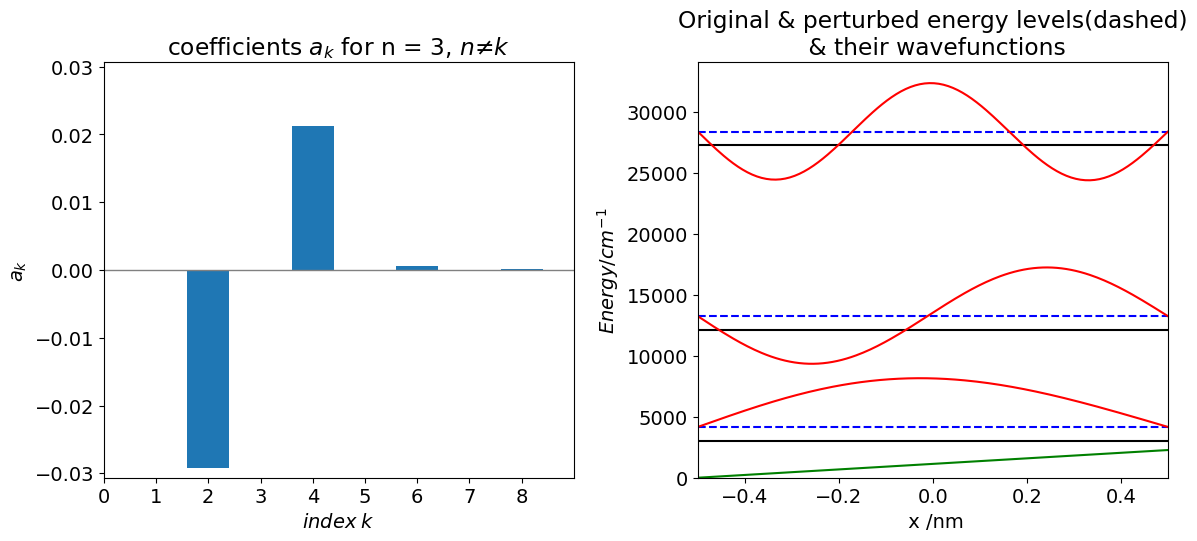
../_images/chapter-5-perturbation-A_6_1.png

Figure 13. Left Coefficients for the \(n = 3\) level and right, original energy levels (solid black), perturbed energies (blue dashed) and wavefunctions for \(n =0, 1, 2\). The green sloping line shows the perturbation.

Applying Maths in the Chemical & Biomolecular Sciences

8 Perturbation Theory

Contents