
Solutions Q1 - 21
Contents
Solutions Q1 - 21#
# import all python add-ons etc that will be needed later on
%matplotlib inline
import numpy as np
import matplotlib.pyplot as plt
from scipy.optimize import fsolve
from sympy import *
init_printing()                      # allows printing of SymPy results in typeset maths format
plt.rcParams.update({'font.size': 14})  # set font size for plots
Q1 answer#
Following the example of the harmonic oscillator, the equation becomes \(v^2 - \omega^2x^2 = c\). This is the equation of hyperbolae and has a saddle point at \(\omega\cdot x\) = 0. The plot is of \(v\equiv dx/dt\) vs \(\omega x\) with arbitrary values of \(\omega\) and \(c\) that we can choose. The figure shows the plot by choosing \(\omega = c = 1\). Different values alters the ‘look’ of the plot, extending in one direction or the other but it always has the same form.
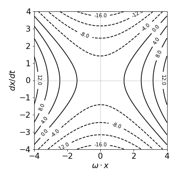
Fig. 31 Phase portrait for \(d^2x/dt^2 - \omega^2x = 0. \quad \omega = c = 1\).
Q2 answer#
(a) \(\displaystyle \frac{dy}{dx}=\frac{xy}{1-x^2}\) or \(\displaystyle \int\frac{dy}{y}=\int\frac{x}{1-x^2}dx\).
Integrating produces \(\ln(y)=-\ln(x^2-1)/2+c\). When \(y_0=c,\; x = x_0\)
and then \(\displaystyle \ln\left(\frac{y}{y_0}\right)= \ln\left(\frac{x_0^2-1}{x^2-1}\right)/2\)
which can be simplified further to \(\displaystyle \frac{y}{y_0}=\sqrt{\frac{x_0^2-1}{x^2-1}}\).
(b) \(\displaystyle \frac{dy}{dx}=e^x\tan(y)\) or \(\displaystyle \int \frac{dy}{\tan(y)}=\int e^xdx\). integrating produces \(\displaystyle \ln(\sin(y))=e^x+c\).
When \(y_0=c, \; x=x_0\) then \(\displaystyle \ln \left( \frac{\sin(y)}{\sin(y_0)} \right)=e^x-e^x_0\)
(c) Rearranging and integrating gives \(\displaystyle \int_0^ye^ydy=\int_0^x e^x\sin(x)dx\), where the limits are included in the integral. The right-hand side can be integrated by parts; the final result is
Q3 answer#
In a bimolecular reaction,when both species have the same initial concentration or the scheme is 2\(A\) \(\to\) product, then the rate equation is
where \(A\) is the concentration at time \(t\), and the initial conditions \(A(0) = A_0\). Integrating produces
which produces
and a plot of reciprocal concentration vs. time is linear. The reaction can also be solved by considering that an amount \(x\) reacts at time \(t\) if \(a\) is the initial concentration then
producing \(\displaystyle \qquad\frac{1}{a-x}-\frac{1}{a}=k_2t\).
Q4 answer#
(a) The integration produces
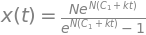
and with the initial condition and some rearranging \(\displaystyle x=\frac{N}{1+(N-1)e^{-Nkt}}\).
As a check, at zero time \(x = 1\) and at long times \(x \to N\). The reason that \(x = 1\) at time zero is that at least one individual must be infected. At long time all are infected. The same calculation using SymPy is a little involved as the initial conditions have to be treated separately.
x, t, k, N, C1 = symbols('x, t, k, N, C1' )       # use SymPy , define symbolic variables
x = Function('x')
f01 = Derivative( x(t),t) -k*x(t)*( N - x(t) )    # eqn 7
ans = dsolve(f01 )
ans
ans1 = ans.subs(t,0).subs(x(0),1)   # substitute with initial conditions
ans1

c1_s = solve(ans1,C1)               # solve for constant
c1_s

simplify( ans.rhs.subs(C1, c1_s[0] ) ) # substitute and simplify

(b) The time for half the population to be infected occurs when \(x = N/2\) giving \(t_{1/2} = \ln(N − 1)/Nk\). This makes sense if \(k\) is small then the spreading of the disease is slow and \(t_{1/2}\) large, and if the population is large it also takes some time for half of them to become infected.
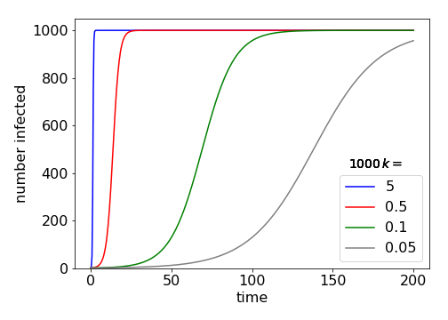
Fig 31-B Example plots of how the number of infected individuals increases with time for different rate constants, \(k\).
Q5 answer#
Scattering takes the place of absorption in the case of X-rays. According to the text, Section 1.11, the scattering cross section for each of \(n\) electrons is \(\sigma = 4\pi e^2/mc^2\). Following reasoning in the text leading to the Beer-Lambert law,
and when the scattering is small the exponential can be approximated giving \(I_s/I_0 = \sigma nL\). For one electron, the amount scattered is \(nL\) times less giving the required answer.
Q6 answer#
The force downwards is \(mg - kv^2\) and the equation of motion is
which using the abbreviation \(b^2=k/mg\) gives \(\displaystyle m\frac{dv}{dt} = g(1 - b^2v^2)\). The solution to this equation is given by
which produces \(\tanh^{-1}(bv)= b(t+c)\).
The hyperbolic tan can be be converted to log form with the standard identity \(\displaystyle 2\tanh^{-1}(ax)=\ln\left( \frac{1+ax}{1-ax}\right)\), hence the result is
To evaluate the constant when the initial velocity \(t_0\) is not zero produces a complicated expression, which only evaluates to a number and so it is left as \(c\) for clarity. It is effectively a displacement in time. Rearranging to find the velocity gives
At long times, the limiting velocity is \(v_{term} = 1/b = \sqrt{gm/k}\). The larger \(k\) is, the smaller the velocity on reaching the ground; a typical value would be \(1000\) kg/m making a terminal velocity for a \(70\) kg skydiver \(\approx \) 0.8 m/s.
Q7 answer#
Differentiating both sides with respect to \(t\) gives, \(\displaystyle \frac{dx}{dt}\left(\frac{1}{a-x}+\frac{1}{(a-x)^2} \right)=ak\),
which simplifies to \(\displaystyle \frac{dx}{dt} = k(a - x)^2\). This means that the rate equation has the form of \(da/dt=ka^2\) because a moles of A and B are present and \(x\) moles react at time \(t\). As a check, if the scheme is
the rate equation is \(d(a - x)/dt = -k(a - x)^2\) which is the same equation as just obtained. The rate constant \(k\) has second order units, \(\mathrm{dm^3\, mol^{-1}\, s^{-1}}\).
Q8 answer#
Newton’s law of cooling is
if \(\theta\) is the temperature of the water and \(\theta_s\) the surroundings. Integrating with the initial condition that at \(t = 0, \,\theta = \theta_0\) gives
The initial temperature is \(15^\mathrm{o}\), the surroundings \(-12^\mathrm{o}\), and the fall is \(5^\mathrm{o}\) in \(8\) minutes, then \(\theta_T = 10\). The rate constant \(k\) is
To form ice the temperature must be zero (\(\theta_T = 0\)) or lower, so that \(\displaystyle t=\ln(27/12)/k = 31.7\) mins.
Q9 answer#
The process is solid \(\to\) vapour and is first order because it is proportional to the amount of solid remaining at any time. If \(s\) is the amount of solid I\(_2\) then the rate equation is \(\displaystyle \frac{ds}{dt} = -ks\) which integrates to \(\displaystyle s = s_0e^{-kt}\) if \(s_0\) is the initial amount of iodine. The rate equation for the amount of iodine vapour is
and integrating with \(s_V=0\) initially produces \(\displaystyle s_V=s_0(1-e^{-kt})\).
The pressure is related to the concentration and using the ideal gas law gives \(s_V = pV/RT, \; s_0 = p_\infty V/RT\) and therefore the pressure increases as \(\displaystyle p = p_\infty(1 - e^{-kt})\).
Q10 answer#
(a) The fluorescence yield is the rate of emission divided by the rate of absorption. This is \(\varphi = k_f /(k_f + k_S)\), equation (5). With quencher the scheme is,
Using \(S_1\) to represent the concentration \([S_1]\) etc., at steady state,
therefore as the fluorescence yield \(\varphi\) is the rate of emission (\(k_f S_1\)) divided by rate of absorption (\(k_aG\)),
Forming the ratio \(\varphi /\varphi_Q\) produces the Stern - Volmer equation with \(k_{\mathrm sv} = k_q /(k_f + k_S)\).
(b) The fluorescence lifetime is by definition the reciprocal of the sum all rate processes destroying the excited state, therefore \(\tau_q=(k_f+k_S+k_qQ)^{-1}\) and in the absence of quencher, \(\tau=(k_f+k_S)^{-1}\). The ratio of these two lifetimes gives a second Stern - Volmer equation
Q11 answer#
The rate equations are
if \(A\equiv [A],\; B\equiv [B]\). The concentration of A is \(\displaystyle A=A_0e^{-k_1t}\) and putting this back into the second rate equation gives
Integrating produces \(\displaystyle B=-A_0e^{-k_1t}-k_0t+c\).
The initial condition is that \([B]_0=0\) therefore,
The maximum occurs when
which gives \(\displaystyle t_{max}=\frac{1}{k_1} \ln \left(\frac{k_1A_0}{k_0} \right)\).
The maximum B concentration is at \(\displaystyle B_{max}=A_0-\frac{k_0}{k_1}-k_0t_{max}\).
(b) Using the values in the question, \(t_{max} = 0.68\) hour and \(B_{max} = 0.99\,\mathrm{ g\, dm^{-3}}\). The time to reach a blood alcohol level of \(B_c = 0.8\,\mathrm{ g\, dm^{-3}}\) is found from \(\displaystyle B_c = A_0(1 - e^{-k_1t}) - k_0t\), which is transcendental and has to be solved numerically. However, the time can be obtained approximately, when \(k_1t\) is large and is then \(B_c \approx A_0 - k_0t\), and is \(\approx 1.9\) hours. Using the Newton - Raphson method the more accurate result is \(1.93\) hours.
The calculation using Sympy is shown below and the generic figure shows the change with time.
# define function to solve numerically
#---------------------
def f(t):
    return Bc - A0*(1.0 - np.exp( -k1*t)) + k0*t
#----------------------

Bc = 0.8              # parameters
k1 = 5.0
k0 = 0.19
A0 = 70.0/60.0
t0 = [0.1 ,2.5]             # initial guesses
roots = fsolve(f, t0)
print('{:s} {:f} {:s} {:f} {:f} '.format('times at conc', Bc, 'are ',roots[0],roots[1] ) )
times at conc 0.800000 are 0.260492 1.929428
Fig32. The equation \(\displaystyle B=A_0(1-e^{-k_1t})-k_0t\) plotted with values given in the question. The concentration is in mg/dm\(^3\) thus a line at \(0.8\) is equivalent to \(80\) mg/ml blood alcohol (dashed horizontal line). In Scotland the legal limit is lower than England and is \(50\) mg/ml blood alcohol (dotted line) , meaning that one would be ‘over the limit’ by far more and for far longer than in England.
When no alcohol remains the residual level is zero, and this occurs \(6\) hours \(8\) minutes after starting to drink. The graph of the time profile of alcohol in the blood is shown in Fig. 32. Because the amount of alcohol decreases linearly with time, at least when the amount is moderate, this can easily be used to back calculate how much alcohol was present at an earlier time. You can see how the model fails when B is small; it predicts a negative B will occur. At very low alcohol levels the reaction is no longer zero order but bimolecular and the concentration does not become negative.
Q12 answer#
The total flux into the pellet is, \(\displaystyle J=+4\pi r^2D\frac{dc}{dr}\)
and is positive as diffusion is into the pellet with a surface area of \(4\pi r^2\). Defined as total flux, \(J\) has units of mole s-1. As the catalyst poisons to radius \(r_p\), then its concentration is given by
If the flux into the pellet is equal to the rate of reaction then \(J = kc_p\), which after rearranging gives,
To see what this function looks like, it can be rearranged to
where \(x\) is a fraction of the radius \(r_p=(1-x)r_0\) and \(\alpha= k/(4\pi Dr_0)\). Two curves are shown in Fig. 33 when \(\alpha \gt 1\) and when \(\lt 1\). When \(\alpha \lt 1\), this means that the diffusion coefficient is large or the rate constant \(k\) small. The concentration of the poison in the pellet is more than 50% almost over the whole volume of the pellet. When diffusion is slow, or the rate constant is large, the concentration of the poison decreases rapidly away from the surface and more than \(50\)% poisoning only occurs within about 10% of the surface.
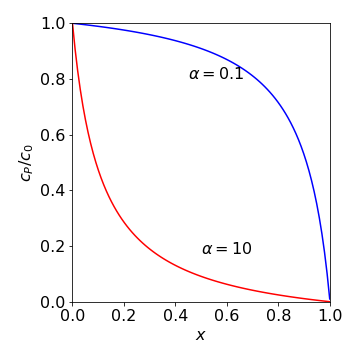
Fig. 33 Relative or fractional concentration of the poison vs. the fraction of the pellet’s radius at two different values of \(\alpha\). The value \(x\) = 0 means that \(r_p = r_0\) and \(x\) = 1 means that \(r_p\) = 0.
Q13 answer#
As M and Q react, the rate is \(\displaystyle k_2MQ = JM = +4πr^2DM \frac{dQ}{dr}\).
To find \(J\) the last two terms are integrated from \(r = R\) to infinity,
which gives \(J=4\pi DRQ\). Equating this to the rate produces the diffusion controlled rate constant \(k_2=4\pi DR\).
Q14 answer#
The rate equation is \(\displaystyle \frac{dR}{dt} = k_IM + (\alpha - 1)k_BR + k_pR - k_pR - k_TR\)
and for clarity we use \(R\) to represent \([R\cdot]\). The propagation step cancels out because in this step one radical is produced for each one consumed. The branching step has the term \(\alpha\) - 1 because one radical is lost accounting for propagation itself. The integral equation when the radical concentration is zero initially is
where \(\gamma = (\alpha - 1)k_B - k_T\). Integrating produces \(\displaystyle \ln\left(k_IM+\gamma R \right)-\ln(k_IM)=\gamma t\) which is more conveniently written as
When \(\gamma \gt 0\), this means that the branching rate constant is larger than the termination one \((\alpha - 1)k_B \gt k_T\), and an explosion could occur because the term \(\gamma t\) in the exponential is positive. However, the rate is limited somewhat at early times, when \(\gamma t\le 1\) and thus there is a short induction period, but after this time is over the radical concentration increases very rapidly and hence the rate of reaction increases rapidly also.
The reaction is stable when \(\gamma \lt 0\) and reaches a steady state at long times; \(R_\infty = k_I M/\gamma\), and this limit is shown in the figure as the horizontal line. The time to reach steady state is the induction period. When \(\gamma \to 0\) the reaction is on the border between stability and explosion and the radical concentration increases linearly with time and to show this we expand the exponential in \(\gamma\) or use L’Hopital’s rule and find \(R = k_IMt \). The condition \(\gamma =0 \) is called ‘chain ignition’.
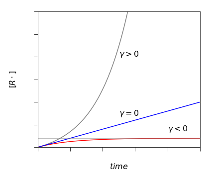
Fig. 33a. The radical \(R\cdot\) concentration under different conditions of chain branching determined by \(\gamma = (\alpha - 1)k_B - k_T\). The steady state limit is shown by the horizontal line.
Q15 answer#
(a) Equilibrium is rapidly established with the complex IM and its rate of change can be taken to be at steady state, hence
giving \(\displaystyle [IM]=\frac{k_1[I][M]}{k_{-1}+k_2[I]}\). The appearance of I\(_2\) molecules is
Integrating this expression with the initial condition that \([I] = [I]_0\) at zero time gives,
which explains the linear dependence of \(1/[I]\) with time.
(b) If each of the rate constants follows an Arrhenius type expression \(\displaystyle k_a = k_0e^{-E_a/RT}\) with activation energy \(E_a\), then, from the rate expression the term \(k_2k_{-1}/k_1\) gives the overall reaction an activation energy \(E_2 + E_{-1} - E_1\). If \(E_1\) is greater than the other two, then the experimentally measured activation energy is negative even though each step has a positive or zero activation energy as must always be the case.
Q16 answer#
(a) The scheme is solvable if \(x\) is the amount consumed at time \(t\),
in which the variables are separable. The initial conditions are \(x = 0\) when \(t = 0\) producing the integration,
This is a standard integration (see Chapter 4) and evaluates, after rearranging, to
which demonstrates how the amount of \(x\) increases from zero to a constant value as equilibrium is approached.
(b) The equilibrium amount \(x_e\) is found when \(t \to \infty\), or using the rate expression when the rate of change is zero, \(k_1(a-x_e)-k_{-1}(b+x_e)=0\), from which
and hence
(c) The amount \(x=\alpha_t -\alpha_0\) and \(x_e =\alpha_\infty -\alpha_0\) then
Because the change with time is proportional to the ratio of the measured quantity, the units of this do not matter because they cancel out. This is always the case for first-order reactions.
(d) The same rate expression in (a) written in terms of the change \(\Delta x=x-x_e\) is
which simplifies to
When integrated, this produces
showing that the relaxation is first-order.
(e) Using the rate constant from the last parts of the calculation and the expression for the rate constant given in the question, produces
The \(\pm V/2\) arises because the potential is zero in the centre of the membrane and is therefore \(-V/2\) on one side and \(+V/2\) at the other. When \(V = 0\), the rate constant \(\displaystyle k = 2k_0e^{-E_0 /RT}\) and this is its minimum value as \(\cosh(x)\) has an approximately parabolic shape. Using the value \(V = 0.1\) eV given in the question, produces \(\cosh(9.6/(2RT)) \approx 3.5\).
Q17 answer#
Let \(x\) be the amount of H+ and OH- ions and \(a\) the concentration of water, then the rate equation is
This equation is separable and can be integrated with the initial conditions \(x\) = 0 at \(t\) = 0 but the result is complex. Changing \(x\) to \(\Delta x + x_e\) makes the equation into
As the perturbation \(\Delta x\) is small, then \(\Delta x^2\) is smaller and can be ignored as it is less than \(2x_e\Delta x\) and \(x_e^2\) and this produces
To eliminate \(a\), use the rate equation at equilibrium \(dx/dt = 0\) to obtain \(k_1(a - x_e) = k_2x_e^2\). The final equation is
which is a first-order equation with solution
where \(x_0\) is the initial change recorded in the experiment and \(k = k_1 + k_2x_e\). It does not matter what units \(\Delta x\) is measured in, because it can always be written as the ratio \(\Delta x/\Delta x_0\) when solving for the rate constant.
Q18 answer#
(a) If \(x\) is the acetone concentration (species A), the rate equation is,
which can be integrated using partial fractions;
which produces two log functions when integrated. The initial conditions are \(x = a_0\) when \(t = 0\) then the integration constant is \(\ln(a_0/b_0)\) and the rate equation,
and the absolute value is added because the log cannot be negative. Rearranging produces
This and also the increase of \(B\) are plotted in Fig. 34.
(b) The phase portrait is an inverted parabola; see Fig.34, Right. The right-hand equilibrium point is unstable, so that from any starting value, \(x\) will end up at zero which means complete reaction occurs. The stability is determined by \(d^2x/dt^2\) and is positive at \(x = a_0 + b_0\), so this point is unstable and negative at \(x = 0\) which is a stable point.
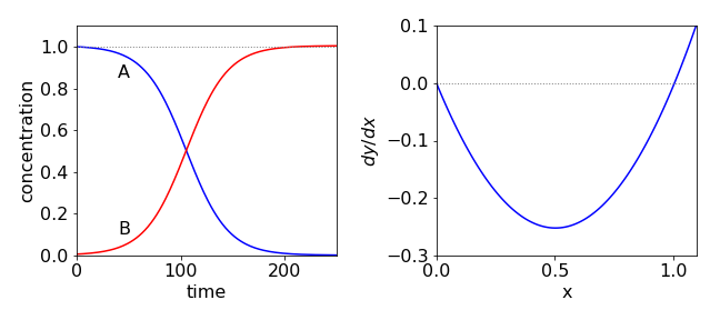
Fig. 34 Autocatalysis. Initially species A decreases slowly as the concentration of B is small. As the reaction proceeds, more B is produced and although A is reduced overall, the rate increases and A is consumed even more rapidly. At longer times, the concentration of A becomes so small that even though that of B is large the reaction rate is slow. The phase portrait is shown on the right.
Q19 answer#
(a) Rearranging gives
at first seems rather hard. Using the substitution \(n/a = e^u\), produces \(dn = ae^udu\) and
Substituting back and adding the limits gives
At long times \(t \to \infty\), the inner exponential becomes very small and as \(\displaystyle e^{-\infty} \to 0\), then \(n \to a\) and the population becomes constant. Therefore, parameter \(a\) must represent the maximum and limiting population. When \(t = 0\), then the population is \(n_0\).
If the initial is less than the final population, this rises gradually to a constant value and the shape of the curve is approximately sigmoidal. If the initial population is greater than \(a\), then the population falls approximately exponentially towards \(a\). The parameter \(k\) is the rate constant (unit = 1/time) controlling the rate at which the final population is reached.
(b) The dimensionless equation is \(\eta = e^{\large{e^{-\tau}} \ln(\eta_0)}\)
where \(\eta = n/a,\; \eta_0 = n_0/a\) and \(\tau = kt\) and the equation is shown in Fig. 35
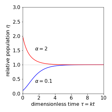
Fig. 35 Population change according to the Gompertz equation.
(c) The equation for \(B\) is found directly and is \(B=Be^{-k_1t}\). Substituting into the equation for \(A\) gives
which can be separated and integrated using the initial conditions;
with the solution \(\displaystyle \ln\left(\frac{A}{A_0}\right)=\frac{k_2B_0}{k_1}\left( 1-e^{-k_1t} \right) \).
This has the form of the Gompertz equation, i.e., \(\displaystyle A = A_0e^{\left((k_2B_0/k_1)(1-e^{-k_1t})\right)}\).
(d) In this model of a tumour, \(k_2 = 1\), if \(B_0\) is the initial rate of tumour growth, \(k_1\) the regression constant and \(A_0\) the number of cells initially present. At long times, \(A \to A_0e^{B_0 /k_1}\) and if the tumour is to shrink then, \(B_0/k_1 \lt 1\) making the exponential less than \(1\).
Q20 answer#
(a) The rate of births is \(k_1N\) and of deaths \((k_2 + k_3N)N\), thus the rate equation is
The steady-state solution is found when the rate of change in population is zero and is either \(N_{ss} = 0\) or \(N_{ss} = (k_1 - k_2)/ k_3\). These are also called the fixed, stationary, or equilibrium points in the phase portrait. If \(dN/dt\) is plotted vs. \(N\), it is zero at the stationary points and in this case, positive in between. For simplicity, the non-zero steady state population is put into the equation and produces,
from which we can see that if \(N \gt N_{ss}\), the population will initially decrease over time; otherwise, it will increase until the steady state is reached, and this is shown in the left-hand pane of Fig. 36.
(b) The rate equation can be integrated by separating variables after first converting into partial fractions. The method is essentially the same as in the previous question. As an illustration SymPy is used here. The calculation is performed in stages as the initial conditions option does not currently work.
k3, N_ss, t, N0, C1= symbols('k3, N_ss, t, N0, C1')   # SymPy define symbols to use
N  = Function('N')
f01= Derivative(N(t),t) - k3*(N_ss - N(t))*N(t)        # define and symbolically solve equation
ans = dsolve(f01)
ans
const = solve( ans.subs(t,0).subs(N(0),N0) , {C1} )   # substitute initial conditions into answer to find C1
const[0]

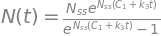
n_t = simplify(ans.rhs.subs(C1,const[0]))       # substitute into initial answer for C1 and simplify
n_t
which can be re-written as
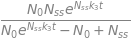
which is more stable numerically as the exponential cannot become very large. With constants \(k_1 = 2,\, k_2 = 1,\, k_3 = 0.001\), and \(N_{ss} = 1000\), with \(N_0\) varying from \(200 \to 2000\) the curves in the left-hand pane of Fig. 36 are produced. As predicted, initially the population rises or falls to the steady-state value. If the rate constant due to over-crowding, \(k_3\), is too large, the steady state population will approach zero.
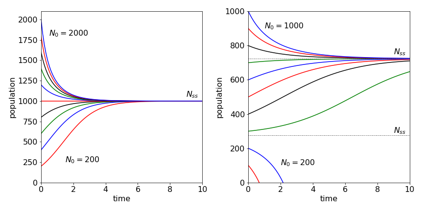
Fig. 36 Left: Population vs. time under ‘normal’ conditions for different initial numbers \(N_0\) increasing by 200 for each curve. Right: Harvesting is introduced with \(k_h=200\) and \(N_0\) values differing by 100 and starting at 100. Notice how the population can crash to zero if the initial number is below the lower of the two steady states, \(N_{ss} \approx 276\). The values of the parameters used are given in the text.
(c) The rate equation is
and the steady state is the solution of \(k_3 N^2 - (k_2 - k_1 )N + k_h = 0\) which is
In the question, \(k_1 - k_2\) = 1 (unit: time\(^{-1}\)), \(2\sqrt{k_3k_h}\) = 0.89 making \(N_{ss}\) = 723 and 276 if \(k_h\) = 200 (unit: number . time\(^{-1}\)). (As \(N_{ss}\) must be a real positive number \((k_1 - k_2)^2 \ge 4k_3k_h\)).
However, solving the rate equation and plotting the values tells another story. At a low initial population as time passes, harvesting may destroy the population and then it becomes negative! The phase portrait allows this to be visualized, Fig. 37. If the initial population is less than the lower critical point, at \(N = 276\) the population moves towards zero because this point is unstable. If the initial population is above this then the second stable point is reached at \(N = 723\) as this point is stable. Thus, to determine whether the population will crash for a given set of parameters, the rate equation does not have to be solved but only the phase portrait examined. However, if you want to know how long it will take the population to crash or to recover, then the rate equation has to be solved.
Fig. 37 Phase portraits for the two population models. The lower curve (blue) corresponds to the model with harvesting. The circles indicate the steady state values; the arrows indicate how the population changes with time depending on its initial value.
Q21 answer#
(a) The singlet states decay by fluorescence and crossing to the triplets and formed by triplet annihilation.
In the rate equation for the singlet state, because two triplets are indistinguishable from one another their amount must be halved. Under the conditions of the experiment, the triplet state rate equation can be simplified to \(\displaystyle \frac{dT}{dt} = -k_aT^2 - k_TT \) which can be solved by separating the variables as
and is integrated by separating into partial fractions. The result is
As the initial condition for the triplet population is \(T(0)=T_0\) the constant can be determined producing
The plot below shows that only at long times does the log plot become linear and gives the correct decay time for the triplet excited state. Rearranging the equation when \(e^{k_Tt}>> 1\) i.e. large gives,
which shows that the decay becomes exponential at long times.
At short times, expanding the exponential produces
which is the equation of a second-order decay process because the reciprocal of the concentration \(T\) is proportional to time. When the annihilation rate constant is small so that \(k_a/k_T <<1\) the decay takes its normal exponential form.
At long times any delayed fluorescence will decay as \(\displaystyle \approx e^{-2k_Tt}\), which is twice as fast as the triplets do, because of the \(T^2\) term in its rate expression. The rate expression is
and letting \(k_f\to k_f+k_s\) for simplicity, and which can be solved using the integrating factor method to give
with the initial value \(S=0\) at \(t=0\). As \(k_f\gg k_T\) the exponential term in \(k_f\) causes the rise in delayed fluorescence to be very rapid compared to its decay. The constant \(c=T_0/(1+k_aT_0/k_T)\). The dashed line in fig 38 shows the decay in the delayed fluorescence when \(k_f+k_s=10^8\, \mathrm{s^{-1}}\) and \(k_T=5000\, \mathrm{s^{-1}}\). The corresponding triplet decays as \(\sim e^{-k_Tt}\) and is shown in green.
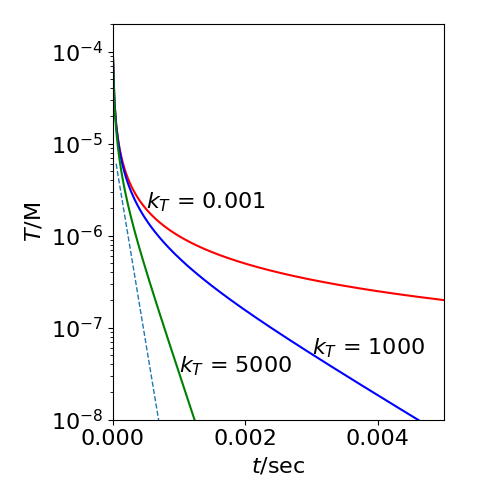
Fig. 38 The decay of the triplet population \(T\) (in \(\mathrm{dm^3\,mol^{-1}\,s^{-1}}\)) vs. time. The effect of T-T annihilation on the T population for different triplet rate constants, \(k_T\) (s\(^{-1}\)) is shown with \(k_a=10^9\,\mathrm{ dm^3\,mol^{-1}\,s^{-1}}\). The initial triplet population is \(10^{-4} \,\mathrm{ dm^3\,mol^{-1}\,s^{-1}}\). The dashed line shows the decay delayed fluorescence at long times, the rise in this is not shown for clarity as it is almost on the vertical axis. The slope is \(-2k_T\) where \(k_T=5000\) and the maximum value has been scaled to fit on the plot.