
Solutions Q49 - 72
Contents
Solutions Q49 - 72#
# import all python add-ons etc that will be needed later on
%matplotlib inline
import numpy as np
import matplotlib.pyplot as plt
from sympy import *
init_printing()                      # allows printing of SymPy results in typeset maths format
plt.rcParams.update({'font.size': 16})  # set font size for plots
Q49 answer#
(a) The centroid in this part has the x-axis as its lower limit hence \(g(x)\) is zero. The limits of \(x\) are \(0 \to r\) the radius.
The second integral can be solved by using a sine substitution which produces \(M_y=r^3/3\) which is by symmetry the same as \(M_x\).
The average \(x\) and \(y\) positions are obtained by dividing the centroids by the area which for a quadrant is \(\pi r^2/4\); see equation 35; \(\langle y \rangle = M_x /A,\; \langle x \rangle = M_y /A\). The average values are \(4r/3\pi\).
(b) In this part \(g(x) = x^2\) then the integrals are
Substituting for the square root using a sine gives the result \(M_x=-(r^2-x^2)^{3/2}/3\) which gives the same value as for \(M_y\), as expected, because of symmetry.
The average \(x\) and \(y\) positions are obtained by dividing the centroids by the area which for a quadrant is \(\pi r^2/4)\); see equation 35; \(\langle y\rangle = M_x /A, \,\langle x\rangle = M_y /A\). The average values are \(4r/3\pi\).
The area is the difference between the two curves, \(\displaystyle \pi r^2/4-\int_0^r x^2dx =\pi r^2/4-r^3/3\) and the average \(x\) and \(y\) values then their centroids respectively divided by the area making the average values \(\displaystyle \langle x \rangle = \frac{(4-3r)r}{3\pi-4r},\, \langle y \rangle = \frac{2(10-3r^2)r}{5(3\pi-4r)}\).
Q50 answer#
(a) The volume of a small circular disc of thickness \(dx\) is \(\pi r^2dx\) where \(r\) is the radius of the disc at any position \(x\). The mass of the element is therefore \(\rho_0\pi r^2dx\) where \(rho_0\) is the density (mass / unit volume) and the total mass of the lens is
The centre of gravity will be on the x-axis \(\langle x\rangle\) from the tip of the lens
which is \(h/3\) from the base. Because the lens is cylindrically symmetric the centre of gravity lies along the x-axis at the point \((2h/3,\, 0)\).
(b) Since now the density is a function only of distance \(x\) then it is uniform in the y-direction. The mass is the integral of the volume element \(\rho_(x)\pi r^2dx\) over the length, which is
The centre of gravity occurs at
This reduces to the previous result when \(b = 0\) and if \(b\) were very large, if such a material existed, then in the limit \(\langle x\rangle = 4h/5\).
Q51 answer#
(a) The volume is \(\displaystyle V=\pi \int_0^\infty y^2dx=\pi\int_0^\infty \frac{dx}{x^2}=\pi\).
The surface area is given by \(\displaystyle S=2\pi\int_a^b y\sqrt{1+y'^2}dx\), where \(y'\) is the derivative.
This gives \(\displaystyle S=2\pi\int_1^\infty \frac{1}{x}\sqrt{1-\frac{1}{x^2}}dx=2\pi\int_1^\infty \sqrt{\frac{x^2-1}{x^4}}dx\). The integration is quite tricky and produces infinity, using Sympy is easy.
x = symbols('x', positive=True)
integrate( sqrt((x**2 - 1)/x**4), (x,1,oo) )

The surface area returned is infinite. This is really a very strange result; in fact, it seems to be nonsensical. The volume is finite therefore the horn can be filled with something, a volume equal to \(\pi\;\mathrm{ dm^3}\) (litres) of paint for example. Its inner surface would be covered but its outer surface area needs an infinite amount of paint to cover it. Repeating the calculation to some finite length, say \(100\), produces a similar result; the surface area is far greater than the volume, but is this not a misleading comparison? The units involved are different. The volume is measured in m\(^3\), area in m\(^2\). Therefore if \(\pi\) litres is used to fill the volume of an infinitely long horn, the surface can be still be covered with this amount of paint but only with an infinitely thin layer. As you will have realized this is not possible. Consider the case when the length is for instance \(9\) dm, and the integral extends from \(1 \to 10\). The area is now \(4.83 \pi\;\mathrm{ dm^2}\) and the volume \(0.9\pi\;\mathrm{ dm^3}\), which means that the coat of paint can now be \(\approx 0.18 \) dm thick.
Exercise: Calculate the surface area of the parabolic lens described in the previous question.
Q52 answer#
(a) As \(p\) is not a variable of the integration and if integration is done first then
Differentiating gives \(\displaystyle F=\frac{be^{-bp}-ae^{-ap}}{p}+\frac{e^{-bp}-e^{-ap}}{p^2}\).
Differentiating first gives
which is a standard form and can be integrated to the same result as above. Using the method above demonstrates an alternative way of evaluating \(\int_a^b xe^{-px}dx\) instead of by parts.
(b) The average of the distribution is by definition, equation 28, \(\displaystyle \langle x \rangle =\int xe^{-px}dx\big / \int e^{-px}dx\). Integrating first gives
and the log part was split into two terms before differentiating because \(\ln(m/n)=\ln(m)-\ln(n)\).
Differentiating first gives \(\displaystyle F= \frac{d}{dp} \ln\left( \int_a^b e^{-px}dx \right) =\frac{\int_a^b xe^{-px}dx}{\int_a^b e^{-px}dx}\) where the integral is treated as if it were any other function. This calculation shows that \(F = -\langle x \rangle\) and the previous calculation gives its value. Normally limits of \(0 \to \infty\) are used in distributions in which case \(\langle x \rangle =1/p\) and \(p\) must have units of \(1/x\).
Q53 answer#
If \(E = \alpha x^2\) then the derivative/integral is the average with respect to \(x^2\) and is
where the integrals are standard ones and the limits are \(\pm \infty\). This result is not zero because the functions inside the integrals are even. As in the previous question this illustrates an alternative way of calculating integrals.
Q54 answer#
(a) The average value of \(E\) is based on equation 28,
and both integrals are ones met before, and are given in the table of integrals. The numerator has the form and gives the average energy \(\langle E\rangle =k_BT\) or \(\langle E\rangle =Nk_BT\) for \(N\) molecules. If \(N\) is Avogadro’s number \(Nk_B = R\), the gas constant, then the average energy per mole is \(RT\).
The mean squared energy is
The numerator has the form \(\int x^2e^{-ax}dx\) which can be integrated by parts. The denominator is \(k_BT\) and so \(\langle E^2\rangle= 2(k_BT)^2\). Using Sympy gives this directly;
E, kB, T = symbols('E, kB, T',positive =True)
eq2 = E**2*exp(-E/(kB*T) )
eq1 = exp(-E/(kB*T) )
integrate(eq2,(E,0,oo)) /integrate(eq1,(E,0,oo))

(b) Using the results just calculated the variance of the energy is
and the standard deviation compared to the average energy is \(\sigma_E /\langle E\rangle = 1\), which, for calculated for a single molecule is a huge fluctuation in energy. This is not observed in practice because of the huge numbers of molecules in a mole. Thus for \(N\) molecules \(\sigma_E^2 = \langle E^2\rangle - \langle E\rangle^2 = (Nk_BT)^2\) and then
Calculated in a slightly different way, the variance is related to the heat capacity as \(\sigma_E^2 = k_BT^2C_V\) and therefore \(\sigma_E \approx \sqrt{N}\) because the heat capacity is proportional to \(N\). (In an ideal monatomic gas \(C_V=3Nk_BT/2\)). As the average energy \(\langle E\rangle\) is proportional to \(N\), then \(\sigma_E/\langle E\rangle \approx 1/\sqrt{N}\) and this ratio becomes very small, even when \(N\) is many orders of magnitude smaller than Avogadro’s number.
Q55 answer#
(a) The variable to be differentiated with respect to is not the same as that for integration therefore the differentiation can be placed inside the integration as
(b) Using the chain rule to differentiate \(\ln(y)\) produces \(\displaystyle \frac{d\ln(y)}{dx}=\frac{1}{y}\frac{dy}{dx}\)
or in general for any function \(\displaystyle \frac{d\ln(f(y))}{dx}=\frac{1}{f(y)}\frac{dy}{dx}\).
Differentiating \(1/x\) gives \(-1/x^2\) or \(\displaystyle d(1/x)=-1/x^2\). Applying this to the equation with \(x\equiv T\) gives the quoted result.
(c) Re-writing produces \(\displaystyle E_a=\frac{k_BT^2}{k(T)}\frac{dk(T)}{dT}\). Differentiating and multiplying by \(k_BT^2\) gives
and dividing by \(k(T)\) gives
The first term is the average energy of all collisions, which is the kinetic energy of the molecules. The second term is the average energy of all reactive collisions, which are distributed as the product of the cross section, the energy and the Boltzmann distribution.
(d) The calculation is
This ratio of integrals turns out to be simply \(E_0+2k_BT\) making the activation energy \(\displaystyle E_a= E_0+\frac{k_BT}{2}\).
The reaction \(\mathrm{Ne^+ +CO \to Ne^+ + C^+ +O}\) follows the line of centres model for the reaction cross-section; many other reactions do not although most do exhibit a threshold for reaction. See McQuarrie & Simon (1997, Chapter 28). The calculation with Sympy is
E, E0, kb, T = symbols('E, E0, kb, T',positive = True)
eq2= (E**2 - E*E0)*exp(-E/(kb*T))
eq1= (E - E0)*exp(-E/(kb*T))
simplify( (integrate(eq2,(E,E0,oo)) )/ (integrate(eq1,(E,E0,oo)) ) )

Q56 answer#
(a) The average speed is by definition,
where the second step follows because the distribution is normalised. Substituting produces
which has a form met before but which can easily be recalculated (assuming that a > 0) or looked up in the integration table (Section 2.13). Using Sympy gives
a, u = symbols('a, u',positive =True)
eq = u**3*exp(-a*u**2)
integrate(eq,(u,0,oo))

where \(a=m/2k_BT\) which makes \(\displaystyle \langle u\rangle =\left( \frac{8 k_BT}{\pi m} \right)^{1/2}\).
The root mean square speed is calculate using
which is an integral of the form \(\displaystyle \int u^4e^{-au^2}du =\frac{3\sqrt{\pi}}{8a^{5/2}}\) making the root mean square speed \(\displaystyle \sqrt{\langle u^2\rangle} =\sqrt{ \frac{3 k_BT}{ m} }\).
(b) The most probable speed occurs at the maximum \(P(u)\) and is found by differentiating the speed distribution and setting the result to zero,
from which \(\displaystyle u_{max_p}= \sqrt{\frac{2k_BT}{m}}\) which is the most probable, but not, maximum speed.
The relative speeds are
These values differ as the distribution is not symmetrical and this is because the minimum speed is zero when the molecules have no energy, and the maximum speed, theoretically, is infinite. In practice, the maximum speeds achievable experimentally in a molecular beam are only a few thousands of meters per second.
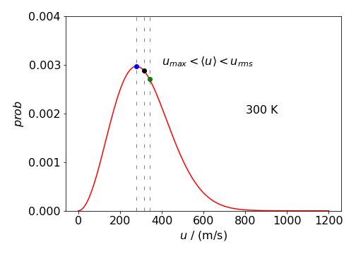
Figure 51b: Boltzmann distribution \(P(u)\) vs \(u\) at \(300\) K for a molecule with the mass of SO\(_2\). The different speeds are marked on the plot. The values are \(u_{max_p}=279,\,\langle u\rangle= 315,\, u_{rms}= 342\) K.
(c) Rewriting the distribution in terms of energy \(E=mu^2/2\) using \(du=dE/\sqrt{2mE}\) and simplifying produces
The average energy is
and the constants cancel. The calculation is a standard one, although producing error functions which disappear on adding limits. The average energy is \(\displaystyle \langle u\rangle =\frac{3}{2}k_BT\) and is the same as requited by the Eqipartition Theorem, \(k_BT\) for each degree of freedom, three in this case because motion is in each of three coordinates, \(,x,\,y,\) and \(z\) The calculation is shown below.
E, kb, T = symbols('E, kb, T',positive =True)
eq32 = sqrt(E**3)*exp(-E/(kb*T))
eq12 = sqrt(E)*exp(-E/(kb*T) )
integrate(eq32,(E,0,oo))/integrate(eq12,(E,0,oo))

With a similar calculation as for the average energy, the mean square energy is
and so the dispersion of the energy is
and the fractional standard deviation \(\displaystyle \frac{\sigma_E}{\langle E \rangle}=\sqrt{\frac{2}{3} }\).
Q57 answer#
(a) The displacement, not the energy, is calculated. The probability function to use is the Boltzmann distribution with the energy at position \(x\). In the harmonic oscillator, it is intuitive that the average displacement is zero; this can also be appreciated from the equation
where the limits are \(\pm \infty\). The numerator is an odd function and, when calculated over a symmetrical range of displacements, is zero, therefore \( \langle x \rangle=0\).
The mean square displacement is not zero as both numerator and denominator are even functions
Both integrals are standard forms and can also be calculated with Sympy in a manner shown in the previous answer, \(\displaystyle \langle x^2 \rangle= \frac{k_BT}{k}\) and hence
Because the average energy \(k_BT\) is fixed at constant temperature, the smaller the force constant \(k\) is, the larger is the spread of the oscillator displacement; exactly as might be anticipated. The average \(\langle x^2 \rangle\) is the average of the square of the displacement from zero either to positive or negative \(x\) and because \(x^2\) is always positive \(\langle x^2 \rangle\) is not zero. The term \(\sqrt{\langle x^2 \rangle}\) is the average displacement.
(b) Using the values given in the question, the root mean square value of the displacement is \(\sqrt{\langle x^2 \rangle} = 4.89\) pm and is a very small percentage (\(1.8\)%) of the bond length of \(267\) pm. This can be taken as the average extension or contraction of the I\(_2\) bond at \(300\) K.
This calculation implicitly assumes that the molecule’s vibrations are not quantised (why is this?) therefore this result is only accurate if the vibrational energy level spacing is small compared to \(k_BT\) when the molecule can be considered to behave classically. As iodine’s vibrational frequency is \(\approx 213 \mathrm{\,cm^{-1}}\) and at room temperature \(k_BT \approx 208 \mathrm{\,cm^{-1}}\), even this heavy molecule, with its small vibrational frequency and energy spacing, should be described by quantum mechanics.
Q58 answer#
The motion is \(x = x_0\cos(\omega t)\) where \(\omega\) is the angular frequency and \(x_0\) the maximum amplitude. The small distance \(dx\) is proportional to \(dt\) and by differentiation
The time \(dt\) taken to go a distance \(dx\) is therefore
and the time for one period is \(T=1/v=2\pi/\omega\). Because \(\cos(\omega t) = x/x_0\), using Pythagoras (right angled triangle) produces
The fractional time to move \(1/2\) a period from \(x_0 \to -x_0\) is therefore, \(\displaystyle \frac{dt}{T}=\frac{1}{\pi}\frac{dx}{\sqrt{x_0^2-x^2}}\).
This equation means that as the fractional time equals the fractional distance, the probability distribution is
This function is approximately ‘U’ shaped about the equilibrium bond extension position. At the maximum extension \(\pm x_0,\, P(x_0)=\infty\) and at \(x=0\) the probability is a minimum and has the value \(1/(\pi x_0)\).
This distribution is infinite at \(x = \pm x_0\) but surprisingly is normalized as can be shown by integrating between the limits of the motion
This is a standard integral \(\displaystyle I=\frac{1}{\pi}\sin^{-1}\left(\frac{x}{x_0} \right)\bigg|_{-x_0}^{x_0}=1\) where \(\sin^{-1}(-1)=-\pi/2\).
(c) The average position is zero because the function to integrate is odd, the probability distribution is symmetrical about \(x = 0\) and the extension and the limits are symmetrical. As the distribution is normalised \(\displaystyle \langle x\rangle = \int xP(x)dx=0\). The mean squared displacement is \(\displaystyle \langle x^2 \rangle = \int x^2P(x)dx\) and is quite an awkward integration. Using Sympy gives \(\displaystyle \langle x^2 \rangle = x_0^2/2\) as shown below. The dispersion, or variance is \(\displaystyle \langle x^2 \rangle - \langle x \rangle^2\) which is also equal to \(x_0^2/2\) because \(\langle x \rangle = 0\).
x0, x = symbols('x0, x', positive =True)
eq = x**2/(pi*sqrt(x0**2 - x**2) )
integrate(eq,(x,-x0,x0 ))

Q59 answer#
(a) The probability distribution function is \(\psi^*\psi dx\) making the integral \(\displaystyle \langle x \rangle = \int_{-\infty}^\infty x\psi^2(x)dx\),
because \(\psi\) is real not complex. First consider the wavefunction for the second quantum level \(\psi_2\), which is an even function, and therefore \(\psi_2^2\) is also even, but multiplying by \(x\) makes \(x\psi_2^2\) odd. Therefore this and all even quantum numbered wavefunctions produce \(\langle x \rangle = 0\).
The odd numbered wavefunctions become even when squared and so these are also zero as \(x\psi_1^2\) is again odd, therefore \(\langle x \rangle = 0\) for all harmonic oscillator wavefunctions. And this is the same result as was obtained classically in the previous example.
Calculating
produces even functions which are not identically zero and have to be evaluated. Using Sympy the first thing to check is that the wavefunctions (Q39) are normalised then \(\int\psi^2 dx=1\).
alpha, x = symbols('alpha, x',positive = True)
psi1 = sqrt(2*alpha)*sqrt(sqrt(alpha/pi))*x*exp(-alpha*x**2/2)
integrate( psi1**2,(x,-oo,oo) )

Next calculate
for a range of \(n\) values. The general harmonic oscillator wavefunction is
where \(\alpha = \mu\omega/\hbar= \sqrt{k\mu}/\hbar\) with reduces mass \(\mu\) and force constant \(k\).
alpha, x, n = symbols('alpha, x, n', positive = True)

def afact(n):     # factorial recursion formula

    if n == 0 or n == 1 :
        return 1
    else:
        return n*afact(n-1)
#------------
def aherm(n,x):   #  Hermite polynomial recursion formula

    if n == 0:
        return 1+0*x
    if n == 1 :
        return 2*x
    else:
        return 2*x*aherm(n-1,x) - 2*(n-1)*aherm(n-2,x)
#------------
ans = []
for n in range(5):
    psi = 1/sqrt( 2**n*afact(n))*sqrt(sqrt(alpha/pi) )* aherm(n,sqrt(alpha)*x) *exp(-alpha*x**2/2)
    r = integrate(x**2*psi**2,(x,-oo,oo ),conds='none')
    ans.append([n,r] )
ans

From these results the general pattern is
for quantum number \(n\) and not unexpectedly the root mean square displacement becomes greater for larger quantum numbers. Substituting for the energy \(E_n=\hbar\omega(n+1/2)=\hbar \sqrt{k/\mu}(n+1/2)\) produces \(\displaystyle \langle x^2 \rangle=\frac{E_n}{k}\) which is similar to the classical value with the quantized energy replacing \(k_BT\), the thermal energy. As Hooke’s law is used describe the extension of a harmonic oscillator within the Schroedinger equation, then it might have been anticipated that \(E_n = k\langle x^2\rangle\).
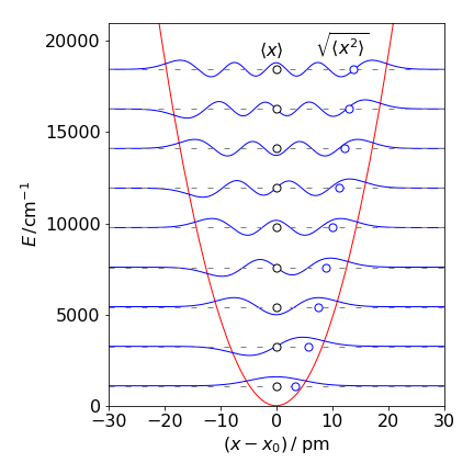
Figure 52. Potential energy and the \(n = 0 \to 8\) vibrational energy levels with the wavefunctions for CO assuming that it is a quantum harmonic oscillator. The equilibrium bond length \(x_e = 0.113\) nm. The average \(\langle x \rangle\) and root mean square distance \(\langle x^2 \rangle\) are also shown as circles.
(e) The average momentum is \(\displaystyle \langle p\rangle =-i\hbar\int_{-\infty}^\infty \psi^*(x)\frac{d}{dx}\psi(x)dx\).
Because the motion is equally to the left and right during the vibration the average momentum should be zero. To check this start with the \(n = 0\) wavefunction \(\psi_0(x)=N_0e^{−\alpha x^2/2}\), where \(N_0 = (\alpha/\pi)^{1/4}\) is the normalization constant. The average momentum is therefore
where and the last step arises because \(xe^{-\alpha x^2/2}\) is an odd function and must evaluate to zero over a symmetrical integration range. A similar calculation for the \(n = 1\) level produces the same result and it can be shown that this result is true for all levels; the average momentum is zero as our intuition dictates.
The square of the momentum, which is proportional to the energy, is not going to be zero because differentiating the wavefunction twice will always produce an even function:
and notice the exponential has also changed. As the function to be integrated is even the integral is not zero.
Using Sympy the result is
after simplifying and substituting for the constants.
x, alpha = symbols('x, alpha', positive = True)
eq =  exp(-alpha*x**2/2)*(alpha*x**2 - 1)*exp(-alpha*x**2/2)
integrate(eq,(x,-oo,oo) )

The previous calculation found that \(\displaystyle \langle x^2 \rangle=\left(n+\frac{1}{2}\right)\frac{1}{\alpha} \) which is \(\displaystyle \langle x^2 \rangle=\frac{1}{2\alpha} \) when \(n=0\).
The product \(\displaystyle \langle x^2 \rangle \langle p^2 \rangle =\frac{\hbar^2}{4}\) and therefore
With states other than \(n = 0\) the uncertainty principle also applies. The harmonic oscillator is somewhat unusual in that the lowest eigenstate exactly matches the uncertainty principle. In many quantum systems, such as particle in a box, each eigenstate has an average position - momentum
Q60 answer#
(a) The distribution is the Poisson distribution multiplied by \(\beta\); see Chapters 1 and 13 for details. The derivation of the distribution assumes many events occur each with a low probability. The energy \(E\) is the expected oscillator energy in units of \(\beta\), and \(s-1\) is the number of oscillators with this energy making \(P\) the probability of obtaining energy \(E\) with \(s-1\) oscillators.
The average oscillator energy is by definition
and if the distribution is normalised then the denominator is unity. It is assumed for the purpose of the question that the averages can be obtained by integration rather than summation. The normalisation is
beta, s, E = symbols('beta, s, E',positive = True)
eqn = beta**s*E**(s - 1)*exp(-beta*E)/factorial(s - 1)
integrate( eqn, (E,0,oo) )

which when simplified has the value unity, because the gamma function \(\Gamma(s)=(s-1)!\). The average is therefore
beta, s, E = symbols('beta, s, E',positive = True)
avE = beta**s * E**s * exp(-beta*E)/factorial(s - 1)
simplify( integrate( avE, (E,0,oo) ) )

where again \(\Gamma(s)=(s-1)!\) is used to simplify. The average energy squared is
The variance is therefore
and the standard deviation \(\sigma =k_BT\sqrt{s}\) where \(\beta=1/k_BT\).
(c) The graph of the distribution is interesting; it becomes more symmetrical as the number of oscillators is increased and the mean value increases, but this is not surprising as the distribution \(P(E)\) is Poissonian and tends to the normal distribution at large \(s\). The average energy when there are \(50\) oscillators is \(s/\beta = 50 \times 200\), which is the same as shown on the graph which was drawn assuming that the energy is a continuous variable. The standard deviation is \(200 \times 50 = 1414 \,\mathrm{cm^{-1}}\).
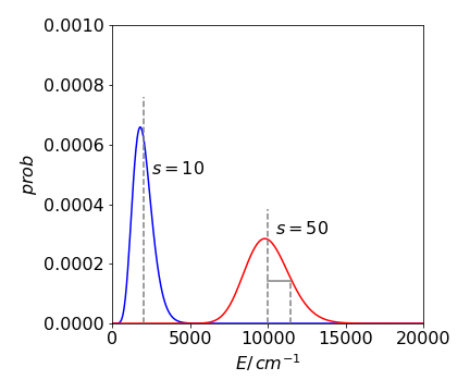
Figure 53. Two probability distributions for \(s\) harmonic oscillators with total energy \(E\) and assuming that the energy is a continuous variable, i.e. classical oscillators. The mean values are shown as dashed vertical lines and \(\sigma\) is shown in the \(s=50\) curve.
Q61 answer#
(a) The normalization is obtained by calculating the probability over all space, which has to be unity, i.e.
and therefore \(\displaystyle N\int_0^L \sin(n\pi x/L)^2 dx=1\). This integral is \(L/2\) as \(n\) is an integer making \(N=\sqrt{L/2}\).
The normalised wavefunction is \(\displaystyle \sqrt{\frac{L}{2} }\sin(n\pi x/L)\)
(b) The average is \(\displaystyle \langle x \rangle =\int_0^L \psi_n^*(x)\,x\,\psi_n(x)dx\)
and should be \(L/2\) as the box is symmetrical about its centre. As a check the integral is
L, x = symbols('L, x', positive = True)
n   = symbols('n',integer=True)
eq1  = 2/L*x*sin(n*pi*x/L)**2
simplify(integrate(eq1, (x,0,L)) )
The average of \(x^2\) depends on the quantum number and is \(\displaystyle L^2\frac{(2n^2\pi^2-3)}{(n\pi)^2}\)
which produces a variance \(\displaystyle \sigma_x^2=\langle x^2 \rangle - \langle x\rangle ^2= L^2\left(\frac{1}{12}-\frac{1}{2n^2\pi^2} \right)\).
and this function is a measure of the spread of the wavefunction. When \(n = 1\) the wavefunction is half a sine wave without a node and most of the amplitude is close to the centre of the box. As \(n\) increases, more nodes are present and the wavefunction spreads out more evenly over the box. As the probability is more evenly spread, the variance \(\sigma_x^2\) becomes larger showing that the wavefunction is less localized.
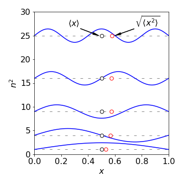
Fig. 54 The first five wavefunctions (\(n = 1\to 5\)) for a particle in a 1 nm box, the mean value of \(x\) and \(\langle x^2 \rangle\) are also plotted. (The energy is plotted as \(n^2\) ignoring the constants, in \(\displaystyle E=\frac{1}{2m}\left(\frac{h}{2L}\right)^2\).
Q62 answers#
Collecting together the terms the equation to use for energy level \(k\) is,
Differentiating the wavefunction twice gives \(\displaystyle -\left(\frac{k\pi}{L}\right)^2\sqrt{\frac{2}{L} }\sin(k\pi x/L)\) making the integral
This integral can easily be evaluated by converting the sine to its exponential form. The result is
Notice that the bigger the box the smaller the energy because the electron is more spread out. Also the larger the mass, the smaller the energy. The calculation in Sympy can be done easily by forcing \(k\) to be an integer.
L, x, hbar, m = symbols('L, x, hbar, m',positive = True)
k = symbols('k',integer = True)

psi = sqrt(2/L)*sin(k*pi*x/L)

simplify(-hbar**2/(2*m)*integrate(psi*diff(psi,x,x),(x,0,L)) )
Q63 answer#
The transition probability can be found from equation 38 and the wavefunctions for the particle in a box,
The initial state has level \(n\) the final \(k\). The average is
and the second integration is identically zero because of the orthogonality of the wavefunctions with different quantum numbers \(n\) and \(k\). The first integral is
To solve this integral convert the sine terms into sums and differences using the trig formula \(2 \sin(a)\sin(b) = \cos(a - b) - \cos(a + b)\) then integrate by parts the two terms produced. Alternatively, the functions can be converted to their exponential form. Using Sympy gives the result directly which is
L, x = symbols('L, x',positive = True)
n, k = symbols('n, k',integer = True, positive = True)

eq = (2/L)* sin(n*pi*x/L)*x*sin(k*pi*x/L)
simplify(integrate(eq,(x,0,L)) )
This equation is zero when \(n + k + 1\) is an odd number. For the HOMO orbital \(n = 4\) and the transitions to other even numbered levels, \(k = 6\) or \(8\) do not occur because \(4 + \mathrm{even} + 1\) is an odd number. Similarly if \(n\) were odd, transitions to other odd numbered levels would be zero. When \(n = 4\) and \(k = 5\) then the average dipole is \(\displaystyle \langle x_{n,k}\rangle = -\frac{160}{81\pi^2}(Lq)^2 \) and the absorption probability, the square of this is \(0.004Lq\). When k = 7 a similar result is obtained which when squared is \(0.00043(Lq)^2 \).
The integrated transition intensity is
where \(\displaystyle \beta = \frac{8\pi^2N}{3000hc}\). Substituting for the frequency, using the energy gap calculated using equations in Q62, the transition frequency is
As the intensity is proportional to \(\nu_{n,k} |\langle \mu_{n,k} \rangle |^2\) and substituting for these terms shows that the intensity is independent of the length of the box \(L\).
The lowest energy transition is
with intensity \(A_{4,5}\approx 0.36\beta\). The intensity of the transition \(4\to 7\) is \(\approx 0.0143\beta\) which is considerably weaker than for the lower energy transition. The reason for this is that the higher wavefunctions have more nodes, but with a smaller period and therefore there is more canceling between the two wavefunctions.
The size of the box cancels out in the intensity calculation because intensity depends only on the shape of the wavefunctions, which is independent of the size of the box. Mathematically the transition frequency is proportional to the inverse of the square of the length and the transition probability to the square of the length and so cancels.
Putting numbers into the constants, the \(4 \to 5\) transition occurs at \(8.52 \cdot 10^{13}\mathrm{ s^{-1}}\) equivalent to \(352\) nm and the \(5 \to 7\) at \(3.12 \cdot 10^{15}\mathrm{ s^{-1}}\) or \(\approx 96\) nm, which are in the right ballpark, but only very approximately correct; experimentally the lowest octatetraene transition is at \(\approx 310\) nm. The model used is very crude and this is not a surprising result because an average bond length was used, and cannot therefore account for alternating bond lengths. Interactions between electrons and nuclei are also ignored. Alternatively, you may consider that the agreement with experiment is rather good considering how very crude the model is!
Exercise: Work out the frequency and intensities of transitions from any of the lower energy levels.
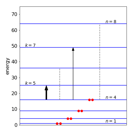
Figure 55. Scaled energy levels in a particle in a box model of octatetraene proportional to \(n^2\), i.e assuming \(\hbar^2\pi^2/(2mL^2)=1\) The allowed optical (dipole) transitions from \(n = 4\) are the arrows, the forbidden transitions the dashed lines. The final state has quantum number label \(k\).
Q64 answer#
(a) If two wavefunctions are not orthogonal then \(\displaystyle \int \psi_a^*\psi_b d\tau \ne 0\).
(b) Using the recursion formula (see answer to Q59)
The third and fourth Hermite polynomials are \(H(2,x)=4x^2-2,\,H(3,x)=8x^3-12x\).
(c) Starting with equation 44 define the wave functions, then calculate the FC factors. First, define the wavefunctions as function of quantum number \(n\) and in terms of constant \(\alpha\), coordinate \(x \)and internuclear separation \(x_0\), and then list them with quantum numbers \(0, \,1\), and \(2\).
alpha, x, x0, x_a, x_b, n, m = symbols('alpha, x, x0, x_a, x_b, n, m',positive = True) #from Q59

def afact(n):                    # factorial recursion formula
    if n == 0 or n == 1 :
        return 1
    else:
        return n*afact(n-1)
#------------
def aherm(n,x):                  #  Hermite polynomial recursion formula

    if n == 0:
        return 1+0*x
    if n == 1 :
        return 2*x
    else:
        return 2*x*aherm(n-1,x) - 2*(n-1)*aherm(n-2,x)
#-------------
def psi(n,x0):
    return 1/sqrt(2**n*afact(n))*sqrt(sqrt(alpha/pi))*\
    aherm(n,(x-x0)*sqrt(alpha) )*exp(-alpha*(x-x0)**2/2)
#--------------

nmax = 3
psin = [''for i in range(nmax)]  # save only to print nicely
for n in range(nmax):
    psin[n] = psi(n,x_a)
    pass

pp = []
for i in range(nmax):            # do this way to simpligy list
    pp.append(simplify(psin[i]))

pp

The lowest energy level has \(n=0\) and its wavefunction, with \(x_0=x_a\) , is \(\displaystyle \psi_0(x,x_a)=\left(\frac{\alpha}{\pi} \right)^{1/4}e^{\alpha(x-x_a)^2/2}\) so that he FC factors from this level to any level \(m\) in state \(b\) are
where the constants are placed outside the integral. Evaluating the integrals with \(m = 0,\, 1, \,5\), and \(6\) and squaring gives
FC = []
for i in [0, 1, 5, 6]:
    ans = integrate(psi(0,x_a)*psi(0,x_b),(x,-oo,oo))
    FC.append([i,simplify( abs( ans)**2) ] )  #  add result to list
FC

Looking at these integrals, notice that the exponential terms are all the same and contain
giving \(FC_{0\to 0} = e^{-X/2}/2\). Looking at the other transitions the constants can be explained as \(\alpha^n/(2^n n!)\) making the general expression
(d) Plotting the FC factors vs quantum number with reduced displacement \(X = 1\) and \(5\), produces the graphs below. When there is a small displacement, most of the intensity of the transition, as controlled by the FC factors, goes into vibrational levels with small quantum numbers of state \(b\), whereas, when the displacement is large, higher state \(b\) quantum numbers are excited Figure 56.
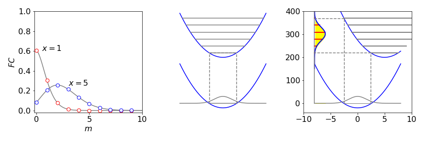
Figure 56. Left: Franck - Condon factors from \(n = 0\) and \(m = 0 \to 10\) in the upper state with reduced displacements of \(X = 1\) and \(5\). Right: The potential energy surfaces with small and large displacements. The dashed lines indicate the range over which transitions can occur. The projection of the ground state wavefunction on the upper potential gives rise to the spectrum only the envelope of which is shown.
Using the exact values for CO, the FC factors, Figure 57 indicate that the excited state is displaced only a little from the ground state. Notice that the envelope of the spectrum is approximately the same shape as the ground state wavefunction but modulated by the FC factors. The spectrum from \(n = 1\) has a very weak \(m = 2\) line compared to \(m = 1\) and \(3\) because the \(n = 1\) wavefunction has one node and therefore very little probability of being near to the centre of the potential.
If the upper state is repulsive and has no discrete levels (bound states), the upper state potential is often so steep that it is approximately a straight line over the small range of overlap of the two potentials. The spectrum is now the projection of the ground state wavefunction potential, see Figure 56.
Exercise: Using the data below, simulate each electronic absorption spectrum. (Herzberg 1950). Investigate increasing the difference in internuclear separation, say by \(10\) to \(50\)%, changing frequencies and starting with levels other than the lowest in the ground state.
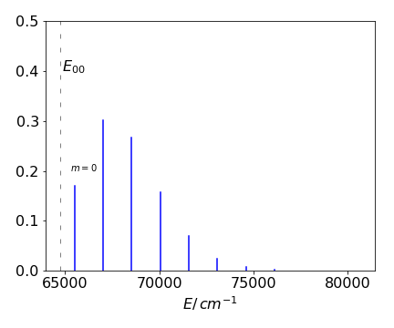
Figure 57. Simulation of the CO electronic spectrum based on calculated Franck-Condon factors from the \(n = 0\) level of the ground state X to \(m = 0 \to 10\) of the A upper state.
Q65 answer#
When \(c=0\) then the only way the donor can lose energy in our model is by fluorescing, hence \(\phi_0 = 1\) because both numerator and denominator in the equation 45 defining \(\phi\) are then the same.
When the concentration is \(c\) then \(\displaystyle \phi=\int_0^\infty e^{-k_ft-(c/c_0)\sqrt{\pi k_ft}} dt\big/\int_0^\infty e^{-k_ft} dt\).
The denominator evaluated to \(1/k_f=\phi_0\), see equation 29. Using Sympy for the more complicated integral with \(a=c/c_0\) gives
kf, a, t = symbols('kf, a, t', positive = True)
eq = exp(-kf*t - a*sqrt(pi*kf*t))
simplify(integrate(eq,(t,0,oo)) )

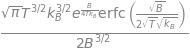
which produces the ratio \(\displaystyle \frac{\phi}{\phi_0}=1 -\frac{\pi c}{2c_0}\text{erfc}\left( \frac{\sqrt{\pi}c}{2c_0} \right)e^{\pi (c^2/2c_0)^2}\)
and where the complimentary error function \(\text{erfc(x)}=1-\text{erf}(x)\). If \(x\equiv \sqrt{\pi}c/(2c_0)\) (which is dimensionless) then the equation is simplified to
At low concentration \(c \to 0\) and hence \(x \to 0\) but as the relative concentration \(x\) is increased, the fluorescence yield of donor molecules must be reduced, because there is always a quencher nearby and \(\phi\) can approach zero. See question Q66 for a calculation of this limit.
At large values of \(x \approx 10\), the error function is so close to unity that an erroneous result is produced. The reason is that the error function, which is an integral, has to be evaluated numerically as does the exponential which is calculated as a series. In this calculation, alternate positive and negative terms cancel out leading to rounding errors. See Chapter 11. The way to overcome this is to use an alternative expansion formula for large \(x\), see figure legend.
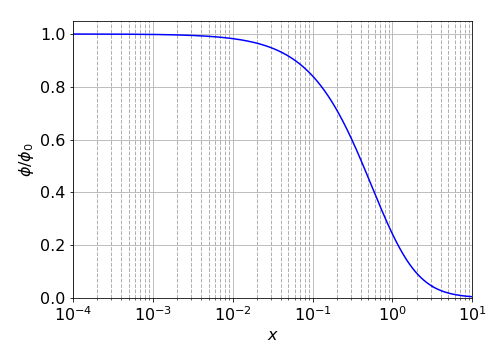
Figure 58. Calculated relative yield of energy transfer quenching on a semi-log scale from \(x = 10^{-4} \to 10\). For \(x\gt 1\) the approximation \(\text{erf}(x)\approx 1/\sqrt{\pi}\left(1/x -1/(2x^3) +3/(4x^5) -15/(8x^7)+105/(16x^9)\right)\) was used (E. Weinstein, Mathworld).
Exercise: Calculate the relative average fluorescence lifetime \(\langle \tau \rangle / \langle \tau_0 \rangle\) vs concentration, see equation 29. Plot the result vs \(x\) and compare the plot with that for the yield.
Q66 answer#
To use l’Hopital’s rule the expression must be put as a fraction, thus
The next step is to differentiate top and bottom separately. The error function is defined as
has the derivative \(\displaystyle \frac{2}{\sqrt{\pi}} e^{-x^2}\). Repeatedly differentiating to and bottom of the fraction separately gives
and consequently the ratio \(\phi/\phi_0 \to 0\).
Q67 answer#
The average depends on \(\theta\) and \(\phi\) and as there are no terms in both angles both integrals can each be separated into a product,
The second integral cancels and the remaining integrals can be done using Sympy or converted to their exponential form:
theta = symbols('theta', positive =True)

numer = integrate(cos(theta)**2*sin(theta), (theta,0,pi))
denom = integrate(sin(theta), (theta,0,pi))
numer/denom

The result is \(\langle \cos^2(\theta)\rangle =1/3\) which proves that
and shows that direct dipole-dipole coupling cannot be measured in solution by using NMR. The spin-spin coupling measured in solution is the indirect dipole-dipole coupling (J coupling) of the nuclear spins mediated via the electrons.
Q68 answer#
(a) The first calculation is to show that the total wavefunction is normalized then by using the definition of an average equation 28 calculate the answers to (b).
Integrating the angular terms in the normalization equation 46 produces
then substituting for the 1s wavefunction gives,
The remaining integral has a form we should identify and has the form,
Substituting for the values
which confirms that the wavefunction is normalised.
(b) As the angular parts of the 1s wavefunction evaluate to \(4\pi\), see (a), the wavefunction being spherically symmetrical, the average \(\langle 1/r \rangle\) is evaluated using
For \(\langle 1/r^2 \rangle\) a similar calculation gives
and \(\langle 1/r^3 \rangle = \infty\) because \(\displaystyle \int_0^\infty \frac{e^{-2Zr/a_0} }{r^n}dr=\infty\) when \(n\ge 1\).
Calculating \(\langle r \rangle, \;\langle r^2 \rangle\) and so forth for positive powers of \(r\) produces the general integral
and the general result is \(\displaystyle \langle r^n \rangle=2^{-1-n}\left(\frac{a_0}{Z}\right)^n (n+2)!\).
n, Z, r, a_0 = symbols('n, Z, r, a_0', positive = True)

eq = 4*(Z/a_0)**3 * r**(2+n)*exp(-2*Z*r/a_0)
simplify(integrate(eq,(r,0,oo) ))

This can be tested and gives finite results only for \(n=-2,\,-1,\,0,\,1,\cdots\)
n, Z, a_0 = symbols('n, Z, a_0', positive = True)
ans = ['' for i in range(7)]
for i,n in enumerate([-2,-1,0,1,2,3,4]):
    ans[i] = (1/2)**(1+n)*(a_0/Z)**n*factorial(n+2)
ans[:]

(c) The standard deviation of a quantity \(x\) is \(\sigma_x=\sqrt{\langle x^2 \rangle -\langle x \rangle^2}\) and for the 1s orbital is \(\displaystyle \frac{a_0}{4}\sqrt{\frac{3}{4}}\), which can be thought of s the uncertainty in the position of the electron. For H atoms this is \(\approx 46\) pm. As \(Z\) increases, this value becomes smaller as the electron is more tightly bound to the nucleus.
(d) The chance of being within any distance \(x\) of the nucleus is the integral from zero up to a distance \(x\), not to infinity, as was used in previous parts of this question;
The integration is done by parts and is simple but involved, instead using Sympy with an upper limit of \(a_0\), gives
Z, a_0, r=symbols('Z, a_0, r',positive=True)

eq = 4*(Z/a_0)**3 * r**2 * exp(-2*Z*r/a_0)
simplify(integrate(eq,(r,0,a_0)) )

This expression evaluates to \(0.323\), thus for the 1s orbital of hydrogen, \(32.3\)% of the electron’s probability lies within the Bohr radius \(a_0\). In a hydrogenic atom with \(Z = 2\) this probability becomes \(76\)% because the electron is more tightly bound. This is shown in the figure for increasing values of \(Z\).
Exercise: Repeat the calculation for any or all of the 2p orbitals. You will need to look up the angular and radial wavefunctions and check that the radial distribution is normalized.
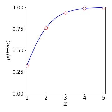
Figure 59. The chance of an electron being within the Bohr radius \(a_0\) for hydrogenic atoms of different nuclear charge \(Z\).
Q69 answer#
The total dipole contribution to the energy of each dipole in the field direction is rather daunting and is
and the average is found by dividing by the integrated distribution giving
The integrals can be solved with the substitution \(a=\epsilon\mu /k_BT\) and \(u=\cos(\theta),\, du=-\sin(\theta)d\theta\). The numerator becomes
The denominator can be treated similarly and produces \(\displaystyle \int_{-1}^1 ue^{au}du=(e^{-a}+ae^{-a}-e^a+ae^{a})/a^2\).
The average energy is the ratio of these last two results and is
Physicists call the term in brackets the Langevin function and substituting for constants gives
Plotting \(\langle E \rangle/\epsilon\mu\) vs \(a\) produces a universal curve as shown in figure 60.
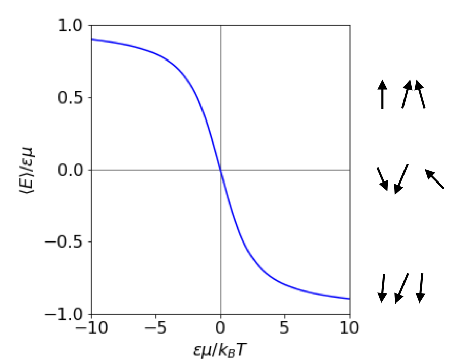
Figure 60 The average dipole energy vs field \(\epsilon\). Both energy and \(\epsilon\) are in reduced units as shown on the axes. The interaction energy is negative when both \(\mu\) and \(\epsilon\) are positive. The lines at \(\pm 1\) show the limiting values at a large positive and negative electric field. At small values of the field the energy varies linearly. The arrows (right) show, in a very diagrammatic way, how the dipoles might align at different field strengths \(E\).
(b) In the case of a small interaction \(\epsilon\mu/k_BT \ll 1\),which means that \(a \ll 1\) and therefore the exponential terms can be expanded as a series \(\displaystyle e^a\approx 1+a+\frac{a^2}{2!}+\frac{a^3}{3!}\cdots \). Using Sympy makes the simple algebra even easier.
a = symbols('a',positive =True)
ans = series( (exp(a) + exp(-a) )/(exp(a) - exp(-a)),a)
simplify( ans - 1/a)

As \(a \ll 1\) then \(a^3\) and higher powers are insignificant therefore the result is for the average energy is
provided that \(\epsilon\mu \ll k_BT\). As a check work out the units. The electric field has units \(\mathrm{J \,C^{-1}\, m^{-1}}\), the dipole C m, so overall the average energy has units of J, which is correct. When the field or dipole is zero so is the energy.
(c) The heat capacity must be a positive quantity and at constant volume is \(\displaystyle C_V=\frac{d}{dT}\langle E\rangle =\frac{\epsilon^2\mu^2}{3k_BT^2}\), which means that \(C_V=-\langle E\rangle /T\) and has units of J/K as expected.
The mean square energy \(\langle E^2 \rangle\) is calculated in a similar way using energy \(E^2\) in the calculations instead of \(E\). Using the substitution \(a=\epsilon\mu/k_BT\), as above,
Then dividing by the normalisation gives
Expanding the exponentials in the limit \(a\ll 1\) gives
which means that this can be re-written in terms of the heat capacity as \(\displaystyle \langle E^2 \rangle=k_BT^2C_V\).
The dispersion or variance at small field values is
and as \(\epsilon\mu/k_BT \ll 1\) then \(\sigma^2 \approx (\epsilon\mu)^2/3\).
The fractional standard deviation at small applied field is \(\sigma/\langle E \rangle \approx k_BT\), which means that the spread of energies is proportional to the temperature. This makes physical sense as the thermally induced Brownian motion of the solvent disrupts the orientational order of the molecule.
(d) At a large field \(\displaystyle \frac{\epsilon\mu}{k_BT} \gg 1\) and the positive exponential terms will dominate \(\langle E\rangle\) then \(\langle E\rangle_{large\, \epsilon} = -\epsilon\mu + k_BT\). When the temperature is low enough or the field large enough, the second term is small compared to the first and the energy is just that of fully aligned molecules \(\langle E\rangle_{large\, \epsilon} = -\epsilon\mu\) as shown in Figure 60.
In calculating \(\langle E^2\rangle\) at large field the exponential terms dominate the other terms and then cancel, and as \(\epsilon\mu \gg k_BT\) it follows that, \(\langle E^2\rangle = (\epsilon\mu)^2\). The variance is \(\sigma^2 = (\epsilon\mu)^2 - (-\epsilon\mu)^2 = 0\) and the relative standard deviation is also zero therefore, when the field is very large the relative standard deviation of orientational energy is zero, i.e. the molecule are perfectly aligned.
Q70 answer#
The average quantum number is, by definition,
The denominator can be integrated very easily by the substitution \(u = J(J + 1)\) the result is \(k_BT/B\). The other integral is far more difficult. It is necessary to spot this otherwise a lot of time would be spent trying to evaluate it; the key is that terms such as \(x^2e^{x^2}\) always involve the error function. Using Sympy gives
B,k_B,T,J=symbols('B,k_B,T,J',positive =True)

eq = J*(2*J+1)*exp(-B*J*(J+1)/(k_B*T))
simplify(integrate(eq,(J,0,oo)) )
making \(\displaystyle \langle J\rangle =\sqrt{\frac{\pi k_BT}{4B}}e^{B/(4k_BT)}\mathrm{erfc}\left( \sqrt{\frac{B}{4k_BT} }\right)\).
Since it is often true that \(B \lt k_BT\), it can be assumed that the error function is zero because \(\mathrm{erfc(small)} \to 1\). In addition, the exponential term can be expanded for the same reason and produces
The numerical value calculated from this last result is almost identical to the full equation at \(600\) K as may be anticipated, because the thermal energy is far greater than the rotational constant; even at \(30\) K, the difference is small. For example \(\langle J\rangle = 1.8\) from an exact calculation and \(1.82\) from the last approximation.
Typical molecular rotational constants are \(1\, \mathrm{cm^{-1}}\) and smaller; exceptions are H\(_2 \,(\approx 60\, \mathrm{cm^{-1}})\) and other diatomics with light atoms HCl for example, \(B \approx 10 \,\mathrm{cm^{-1}}\). In comparison thermal energy at room temperature is \(\approx 208 \,\mathrm{cm^{-1}}\).
(b) The maximum and average values of the quantum number differ because the distribution is not symmetrical, Figure 61. The maximum in the population vs quantum number curve is caused by the increasing degeneracy \(2J + 1\) together with the exponentially falling population with increasing \(J\) given by the Boltzmann distribution.
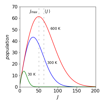
Figure 61. Rotational distribution for Br\(_2\), at \(30, \,300\), and \(600\) K, assuming \(J\) is a continuous quantity. The maximum and average value of the rotational quantum number is shown on the graph at \(600\) K. They differ because the distribution is not symmetrical.
Q71 answer#
(a) Substituting for \(g\) produces
Integration of this form involve the error function and can be started with the substitution \(u=\sqrt{\epsilon}\) and using integration by parts. The error function evaluates to zero and 1 with the limits zero and infinity respectively making the integral;
The translational partition function is \(\displaystyle Z=V\left(\frac{2\pi mk_BT}{\hbar^2}\right)^{3/2}\).
The integration via Sympy is shown below.
epsilon,k,T=symbols('epsilon,k,T',positive=True)
eq = sqrt(epsilon)*exp(-epsilon/(k*T))
simplify(integrate(eq,epsilon) )

Q72 answer#
(a) The expectation has the usual form \(\langle p_x \rangle=\int \psi^*p_x\psi dx\big/\int \psi^*\psi dx\).
The normalisation (denominator) is a constant equal to \(\int dx\) but the numerator is
thus \(\langle p_x \rangle=p_x\).
(b) the expectation is \(\displaystyle \langle p_x^2 \rangle=(-i\hbar)^2\int e^{-ip_x x/\hbar}\frac{d^2}{dx^2} e^{ip_x x/\hbar} dx\big/ \int dx = p_x^2\).
(c) The previous results produce \(\Delta p^2 = 0\) which show that \(\psi\) is an eigenfunction of both operators \(p_x\) and \(p_x^2\). This can also be realized because both operators commute,
The function operated on is a normal function of \(x, \,f (x)\) such as \(\psi\).