Solutions Q13 - 16
Contents
Solutions Q13 - 16#
# import all python add-ons etc that will be needed later on
%matplotlib inline
import numpy as np
import matplotlib.pyplot as plt
from sympy import *
init_printing()                      # allows printing of SymPy results in typeset maths format
plt.rcParams.update({'font.size': 16})  # set font size for plots
Q13 answer#
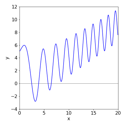
Using the algorithms in the text the following figure can be produced from which it is clear that both the Euler methods fail badly in this instance and even the Runge - Kutta fails when \(t\) is large. If the number of integration points is increased to \(1000\), the Euler methods improve slightly but still fail, however, the Runge - Kutta is essentially identical to the exact solution but only up to about \(t=15\) when it starts to fail badly. This illustrates how difficult, and time consuming numerical calculations can be. Time consuming since very small steps may be needed to ensure accuracy.
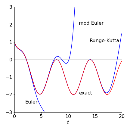
Figure 33. Comparison of the Euler methods with the Runge - Kutta and the exact solution, red line.
Q14 answer#
(i) The code in the ‘for’ loop has to be changed to use the modified Euler equation (33). The derivatives are defined as
dydt = lambda t,x,y : -(kf+k2)*y+k1*x
dxdt = lambda t,x,y : -(k1+ke)*x+k2*y
and using the values given in the question the plot produced is
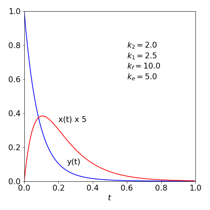
Figure 34. Plots of solution.
The plot shows that initially \(x\) increases from zeros, because it is produced from \(y\), then decays away with rate constant \(k_e\). Equilibrium is beginning to be is set up between \(x\) and \(y\) but this does not last as both species decay with rate constants \(k_f\) and \(k_e\).
(ii) The rate equations are
the algorithm is shown below.
#--------------------------------
def EulerN(f0, f1, t0, y0, z0, maxt, N):         # Euler method, function two rate equations f

    Eulery = np.zeros(N,dtype=float)   # define arrays to hold results  y is molecule type A
    Eulerz = np.zeros(N,dtype=float)   # z is moleculae type B
    dtime  = np.zeros(N,dtype=float)
    h = (maxt - t0)/N
    y = y0                             # initial values
    z = z0
    t = t0
    Eulery[0]= y0
    Eulerz[0]= z0
    dtime[0] = t0
    for  i in range(1,N):              # loop starts
        y = y + h*f0(y,z)              # increment y
        z = z + h*f1(y,z)
        t = t + h                      # time
        Eulery[i] = y                  # save values
        Eulerz[i] = z
        dtime[i]  = t
        #if i == N // 2:               # modification to add more B
        #    z = z + 1*z/5
        pass                           # end of loop
    return Eulery,Eulerz,dtime
#---------------------------------

dAdt = lambda A,B : -k1*A + k2*B**2    # equation to integrate
dBdt = lambda A,B :  k1*A - k2*B**2    # equation to integrate

A_0 = 2.0    # initial pressure
B_0 = 0.0
k1  = 0.17    # values in units microseconds
k2  = 1.0
maxt= 15.0
N   = 400    # number of points
t0  = 0.0

Avals, Bvals, atime = EulerN(dAdt,dBdt,t0,A_0,B_0,maxt,N)   # Call procedure, return values

#fig = plt.figure(figsize=[5,4])        # remove # to plot
#plt.plot(atime,Avals,color='blue')
#plt.plot(atime,2*Bvals,color='red')
#
#Ke = k1/k2
#Ae = ( 2*A_0+Ke  - np.sqrt( (2*A_0+Ke)**2 -4*A_0**2))/2  #  equilibrium amount
#
#plt.axhline(Ae,color='blue',linestyle='dashed',linewidth=1)
#plt.axhline(2*(A_0-Ae),color='red',linestyle='dashed',linewidth=1 )
#
#plt.xlim([0,maxt])
#plt.ylim([0,1.5])
#plt.ylabel('concentration')
#plt.xlabel('time')
#plt.text( maxt-2,1.1*Ae,'[A]')
#plt.text( maxt-2,0.85*2*(A_0-Ae),'[B]')
#plt.tight_layout()
#plt.show()
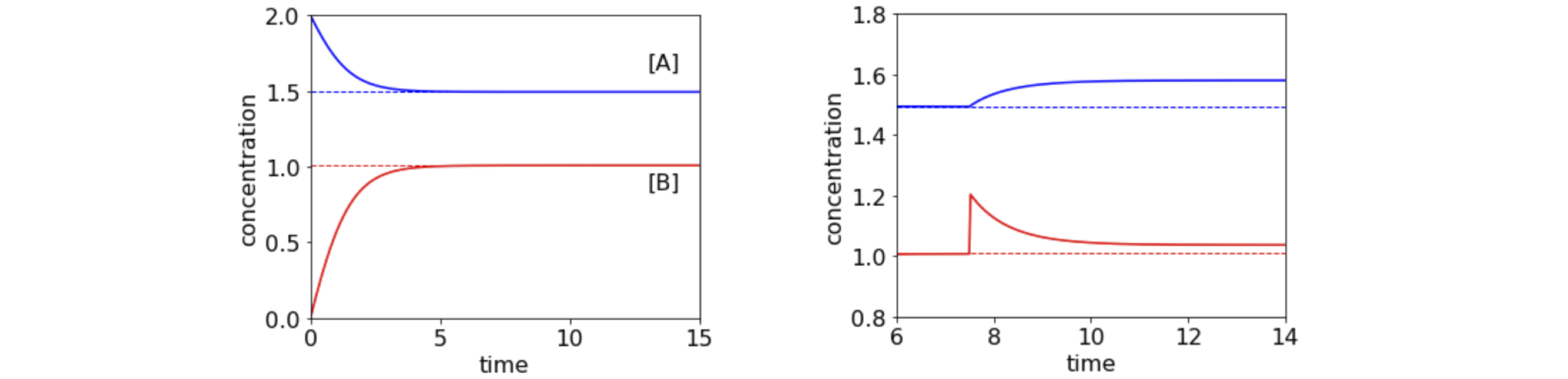
Figure 34a. Left. Plot of concentration of species A and B vs. time showing how equilibrium is reached. The dashed lines show the algebraically calculated equilibrium. Right. Detail shows the effect of adding an amount amount of B when equilibrium has already been reached and its return to a new equilibrium position. Time is in units of microseconds.
(ii) The equilibrium amounts can be found by starting with \(dA/dt\) and as \(A\to A_e\) at equilibrium,
solving for \(A_e\), with \(K_e=k_1/k_2\) as the equilibrium constant, gives \(\displaystyle A_e=\left(2A_0+K_e+\sqrt{(2A_0+K_e)^2-4A_0^2}\right)/2\), which is shown in the plot, and \(B_e=2(A_0-A_e)\).
(iii) If the amount of B is instantaneously increased then there are more molecules overall and both the amounts of B and A will have to increase compared to that before the change. However, just after the change there is too little A for the amount of B now present (because the system was at equilibrium and is transiently not anymore) meaning more A will form from B and so B will decrease until equilibrium is re-established. This is shown in figure 34a. The transient approach to equilibrium has a lifetime of \(\tau =1/(k_1+k_2[B_e])\) or \(0.86\;\mathrm{\mu\,s}\)
Q15 answer#
Four rate equations are needed and are,
The functions in the algorithm can be written as
dSdt=  lambda S,E,ES : -k1*S*E + km1*ES
dEdt=  lambda S,E,ES : -k1*S*E + (km1+k2)*ES
dESdt= lambda S,E,ES :  k1*S*E - (km1+k2)*ES
dpdt=  lambda S,E,ES :  k2*ES
and in the ‘for’ loop as
#for i in range(1,n):                # commented out here only to prevent error as this is a stub.
#    S =  S  + h*dSdt( S,E,ES)
#    E =  E  + h*dEdt( S,E,ES)
#    ES = ES + h*dESdt(S,E,ES)
#    p =  p  + h*dpdt( S,E,ES)
#    t = t + h
#    # etc
The results are shown in Fig 35.
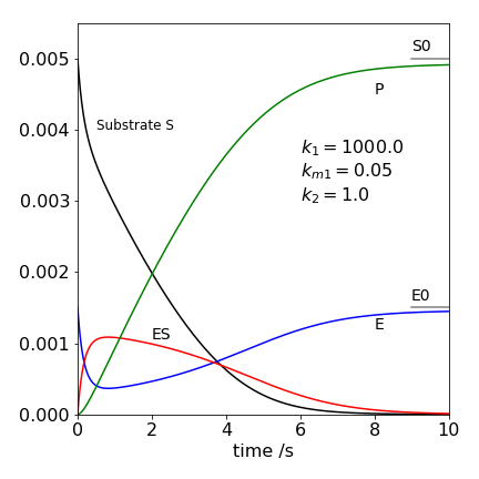
Figure 35 Michaelis - Menten concentration profiles. The intermediate complex ES is represented by the red line.
In the figure we see that the product concentration \([P]\) rises to reach the same concentration as the substrate concentration \([S_0]\) and that the enzyme E after initially reacting returns to its initial concentration \( [E_0]\). The substrate concentration falls rapidly to begin with, then more slowly. This is due to establishing the equilibrium between S + E and ES and therefore ES initially rises rapidly and reached a maximum and falls because it is slowly lost to product. The steady state condition is \(d[ES]/dt = 0\) is only approximately satisfied with these rate constants after ES has reached its maximum and extends only to about two seconds. The calculation clearly shows the approximate nature of the steady state approximation, we assume that the gradient is zero but have to be satisfied that it is small. Notice also that the steady state conditions mean that the concentration of the species ES need not be small, just that its gradient with time is small. This is a common misconception in the steady state approach.
Q16 answer#
Using the substitution \(z = dy/dx\), the equation becomes \(dy/dx=z\) and \(d^2z/dx^2=-xz-y-x\) which has to be split further using \(w = dz/dx\) to give
The equations are added into the calculation as shown in other answers