
9 Sophisticated Counting.
Contents
9 Sophisticated Counting.#
%matplotlib inline
import numpy as np
import matplotlib.pyplot as plt
from sympy import *
9.1 Permutations, Combinations and Probability.#
The branch of mathematics dealing with permutations, combinations, and probability is perhaps that most closely related to everyday experience, particularly so if you play cards or do the lottery. There are different ways of counting the number of the arrangements of objects, such as molecules or footballs and these are permutations and combinations.
(i) Permutations#
Permutations count the number of ways of arranging objects so that each permutation is unique. This means that the order is important.
(ii) Combinations#
Combinations count the number of ways of selecting objects from a group without considering the order of selecting.
We shall describe these quantities in terms of ‘objects’ and ‘boxes’ and let them variously apply to dice, playing cards, electrons, atoms, molecules, and energy levels as the context requires.
In genetics, probabilities are used when calculating the outcome from mixing genes through the generations. In physical science, statistical mechanics uses ideas based on placing particles into energy levels and from their distribution, partition functions can be calculated which in turn lead to thermodynamic quantities.
The probability or chance of an event occurring, will be defined as the ratio of the number of successful outcomes to the total number of possible outcomes, and can only have values from \(0\) to \(1\). It is implicitly assumed that any one event is just as likely to occur as any other. A particular outcome is not therefore predictable; only that a certain fraction of times the expected result will occur if many trials are carried out. For instance, you would not expect to be able to throw a die so that a \(1\) is always produced. One might obtain a \(1\) on the first throw. If a \(1\) is obtained on the second throw, this is surprising, but if on a third, this suggests, but does not prove, that the die might be biased because we expect a die to produce a \(1\), or any of its other numbers, on average only once in six throws. Probability theory allows the calculation of the exact chance of each possible outcome without having to do the experiment. Because the probability or chance of a successful event \(p\), cannot be greater than \(1\), the chance of failure is \(q = 1 - p\).
9.2 Permutations#
A permutation is an ordered arrangement of objects and if the order is changed then a new permutation is produced. The five letters A to E arranged as A B C D E form one permutation; A B C E D and A B E C D are two others. It is implicitly assumed that the each number/letter/object is chosen with equal probability and there is an equal chance of filling any place in the list that is produced. Note that there are no repeated letters, or numbers (objects), in any list.
If there are five different objects (\(n=5\)) then there are \(5! = 5 \times 4 \times 3 \times 2 \times 1 = 120\) permutations. The proof is straightforward: starting with five vacant places in a row, one letter, the letter E, for example, can be put into any one of five different places. There are now \(n-1 = 4\) letters left and if D is now chosen then it can only be placed in four, i.e. \(n-1\) different positions as E occupies one of them. This means that the first two numbers can be placed in \(n(n-1)\) different ways. The third letter chosen can only be put into three (\(n-2\)) empty positions and so the first three numbers can be placed in \(n(n-1)(n-2)\) different ways and so forth. The number of permutations when all \(n\) objects are chosen is therefore the product of the numbers of ways in which to put the letters and this is \(n(n - 1)(n - 2) \cdots 1= n!\). This can easily be a truly vast number, but if there are only three objects then there are only 3! = 6 ways of doing this which are ABC, ACB, CAB, BAC, BCA, CBA and any permutation is distinguishable from all others. The permutation of \(n\) objects is \(n\) objects in \(p=n\) boxes and written as
When only some number \(p\) of the \(n\) objects are chosen, the permutations will be fewer, we effectively stop before \(n\) choices have been made. We saw above that if only two choices are made out of \(n\) the number different choices is \(n(n-1)\). Suppose that either \(p\) objects at a time are chosen out of \(n\), or that \(p\) objects are placed into \(n\) boxes so that no more than one is in any box, then the number of different ways of doing this ‘p from n’ calculation is
Choosing any two letters, \(p = 2\), from three, \(n = 3\) produces 3!/1! = 6 permutations. For example, if the letters are ABC, then the six choices are AB, BA, AC, CA, BC, CB. Because each permutation is distinct, if we were to place them into groups or ‘boxes’ then only one arrangement goes into each box. When \(n = p\), because \(0! = 1\) this equation equals \(P(n, n) = n!\). If each of the permutations is equally likely, then the probability of any one occurring is \(1/P(n, p)\). Finally, note also that the notation \(P(n, p)\) is not universal and \(_nP_p,\; ^nP_p\) or \(P_p^n\) are also commonly used.
If the letter/number/object is removed after being put into a box, so that all boxes are empty, then there are always \(n\) choices and so the total number of different ways becomes \(n^p\) when there are \(n\) boxes and only \(p\) objects. Alternatively, if we imagine that the box is full of letters then in the first case there are \(n\) choices to take the first letter out and \(n-1\) for the second etc., but if the letter is replaced then there are \(n\) each time making \(n^p\) in total.
(i) Permutation Examples#
(a) The number of permutations that can be made, each of 3 vowels long, from a, e, i, o, u is \(\displaystyle P(5,3) = \frac{5!}{2!}=20\)
(b) If five letters are chosen from the alphabet there will be \(\displaystyle p(26,5)=\frac{26!}{21!}=7,893,600\) different ways of forming these groups.
(c) A six digit phone number, where all digits are different, is made up of the digits \(0-9\) inclusive, thus there will only be \(\displaystyle p(10,6)=\frac{10!}{4!}=151200\) different groups.
(d) How many integers are there between \(10\) and \(100\) ignoring those with the same two digits, i.e. \(11,22\) etc? This can, of course, be worked out by simply adding up the integers but the number of them is also found from the number of groups of two different numbers out of the numbers \(0-9\), which is \(\displaystyle p(10,2)=\frac{10!}{8!}=90\). The similar problem of finding all positive three digit integers not containing any repeated digits is \(\displaystyle p(10,3)=\frac{10!}{7!}=720\), much easier than trying to work it out by counting how many of each type there is.
(e) In a race between twelve runners the number of ways that first, second and third places can be awarded is \(\displaystyle p(12,3)=\frac{12!}{9!}=1320\).
9.3 Permutation with groups of identical objects#
If some of the \(n\) objects are identical then clearly the number of choices is going to be reduced. To take an extreme example, if all the objects are identical or indistinguishable from one another, then there is only one way of arranging them and the number of permutations is one. If there are \(n\) objects split into two groups and each of \(v\) and \(w\) are identical objects, the number of permutations is reduced by dividing by the number of ways of separately arranging every identical group, and the result is \(n!/(v!w!)\). If the \(n\) objects are A A B B B E C D, then there are \(8!/(2!3!) = 8 \times 7 \times 6 \times 5 \times 2 \) ways of arranging them or 12 times less than if all the letters were distinct.
The identical grouping permutation can be stated more formally as the number of ways of selecting \(n\) objects if these are in \(r\; (\le n)\) groups of \(m_1, m_2, m_3 \cdots m_r\) objects. The total of all \(m_r\) objects must be \(n\). The number of permutations with groups is
where the symbol \(\prod\) indicates the product. This number is also the number of ways of placing \(n\) distinguishable objects into \(r\) distinguishable boxes so that boxes contain \(m_1,\; m_2, \;m_3 \cdots m_i\) objects each, and each of the objects in any one box is alike.
The number of ways of arranging the amino acid residues of even a small protein is astronomically large, but countable. An active protein in a bee’s sting is called mellitin. It is a protein with only 26 amino acids and which forms two short \(\alpha\)-helical regions, with a bend in between. Two such helices are seen in the crystal structure 2MLT.pdb in the RCSB data base (www.rcsb.org/pdb/home/home.do).
The sequence of the structure is
GLY ILE GLY ALA VAL LEU LYS VAL LEU THR THR GLY LEU PRO ALA LEU ILE SER TRP ILE LYS ARG LYS ARG GLN GLN
Collecting the residues together produces groups of 3 gly, 3 ile, 2 ala, 2 val, 4 leu, 3 lys, 2 thr, 1 pro, 1 ser, 1 trp, 2 arg, and 2 gln and this produces
ways of arranging a chain. Nature has had to search in the ‘space’ of all combinations to find an effective protein (one that causes pain when you are stung) and has had a very long time to do so. However, this number of permutations is still so large that even producing a different sequence at one a minute, supposing that this were possible, would have taken \(\approx 5 \cdot 10^{15}\) years, which is far longer than the age of the Earth. This is a questionable calculation for two reasons at least. One is that it assumes that the protein always had \(26\) amino acids whereas, in the distant past, it was probably far smaller but was nevertheless effective enough to give the bee’s ancient ancestor an evolutionary advantage. Secondly, many permutations of even a few amino acids will not have the stability to form any structure other than a random coil and so could never exist as a functioning protein. Those that do form some stable structure and are effective are then preserved and passed down to the next generation, and by mating and random mutations, improved. (Those that do not offer improvement produce fewer offspring and are eventually after some generations removed from the population). Therefore the whole of the possible permutation space is never searched, but the search algorithm that is natural selection very effectively finds a working solution and one that is usually close to the optimum.
9.4 Combinations#
A combination is really a misnomer, because it is the number of ways of choosing \(p\) distinguishable objects from a group of \(n\) distinguishable objects, and the order of choosing these \(p\) objects does not matter. If two letters from ABC are chosen, the number of combinations is three and the choices or combinations are AB \(\equiv\) BA, AC \(\equiv\) CA, BC \(\equiv\) CB because the order does not matter. If there are five things we can take two of them in ten different ways. If the things are labelled A, B, C, D, E then the combinations of two at a time are AB, AC, AD, AE, BC, BD, BE, CD, CE, DE.
If we think of placing objects into boxes, combinations, unlike permutations, allow more than one object to be placed in each box. For example, the letters ABC can fill three boxes each containing two objects. Removing \(p\) of the permutations is equivalent to dividing the objects into two groups, the chosen group of \(p\) objects and another group, not chosen, containing \(n - p\) objects.
In a permutation, there are \(n!\) ways of choosing (if all the objects are different) and a combination must be less than this because the ordering of similar objects does not matter, and is less by the factorial of the number chosen, which is \(p!\). Four objects A, B, C, D produce \(4! = 24\) permutations. If any three (\(p = 3\)) are chosen at a time, the four combinations \(C(4, 3)\) are ABC, ACD, ABD, BCD. Each of these groups has \(p! = 3! = 6\) permutations making \(4 \times 6 = 24\) permutations in total. Thus the number of combinations \(C\) is
Therefore, using equation 19, the number of ways of choosing \(p\) objects at a time out of a total of \(n\), is
The second notation, ‘n over p’, is that used for the coefficients in the binomial expansion. As for permutations, various notations for combinations, \(_nC_p,\; ^nC_p,\; C_p^n\) are also common. The combination gives the coefficients in the binomial expansion and in the Binomial Probability distribution, see section 9.10.
The original context of the word combination is that the number \(C(n, p)\) is the number of combinations of \(n\) things selected \(p\) at a time. Since \(\displaystyle \binom{n}{p}=\binom{n}{n-p}\) this is also equal to the number of combinations of \(n\) things selected \(n-p\) at a time.
9.5 Lottery#
The chance of winning a lottery can be found from the number of combinations. For instance, choosing 6 numbers out of 48 produces
possible choices or just under one in twelve million chances of winning. As the chance of any one combination being chosen is just as likely as any other, then its probability is \(1/C(n, p)\). If \(\approx 12\) million people play each week, then on average one might expect one winner each week, assuming that the numbers are equally likely to be chosen by the players.
9.6 Choosing groups#
If you are making choices when two or more conditions apply, then the combinations are multiplied together. For example, suppose that a study is to be conducted in which \(25\) patients are to be placed into three groups of equal size. The control group must contain \(8\) persons and therefore so must the experimental groups. These must be selected from \(25 - 8 = 17\) and \(9\) persons each. The number of ways of making this choice is vast even for such small numbers, and is
9.7 Number of transitions#
In a stack of energy levels such as in an atom, many transitions are possible from an upper level \(n_2\) to a lower one \(n_1\) if the selection rules are ignored. Thus level \(6\) can have transitions to levels \(5,4,3,2,1\), level \(1\) being lowest, and level \(5\) can then transfer to levels \(4,3,2,1\) etc. The first step is to calculate the number of levels and this is just \(n_2-n_1+1\). You can check this by drawing a set of levels. Next, each transition, of course, involves two levels so we need to find the number of ways of selecting two levels (objects) at a time out of the total and this is
9.8 Number of determinants in a MO calculation#
In the Hartree-Fock self consistent field method of calculating molecular orbitals the wavefunction is described by spin orbitals that are arranged into Slater determinants (see chapter 7 Matrices). There are more spin orbitals than electrons because the wavefunction is expressed as a series of terms and the more terms included lower the energy. The determinants are used to ensure that the Pauli principle applies, which in its wider sense means that the wavefunction is antisymmetric when any two electron coordinates are exchanged. The calculation can be done with the smallest set of determinants, which means using just the lowest energy spin orbitals, but this does not generate the lowest possible energy. What is done is to make wavefunctions, described by Slater determinants, that correspond to one or more excitations and this lowers the energy. This is fine as far as it goes but the number of possible ways excitations can be achieved is vast, and this is of practical importance as each calculation involves evaluating an integral and so has implications on computer time and memory size. Including excited determinants is called Configuration Interaction. A typical example is that of benzene described by \(72\) spin orbitals and \(42\) electrons.
Instead of thinking of determinants, suppose that there are a number of energy levels, or boxes if you wish, into which particles are placed such that only one is allowed into any level. If, for example, there are \(72\) levels and \(42\) particles what are the number of ways that these can be placed? The number of combinations is \(\displaystyle \binom{72}{42}=\frac{72!}{42!30!}=1.6\cdot 10^{20}\) which is vast. Next, suppose that only the lowest \(42\) levels are occupied how many ways can we move a single particle at a time to an empty level. This would correspond to singly excited determinants and is the number of choices by which one particle can be moved and that is \(30\) and so for all particles is \(42\cdot 30 = 1260\). Now if two are moved at a time (a doubly excited determinant) then the number is \(\displaystyle \binom{42}{2}\binom{72-42}{2}=374535\). The extension to moving three at a time is clear but we cannot move all of them at once because there are more particles than empty spaces. You can appreciate just how many integrals have to be evaluated when calculating benzene’s molecular orbitals.
9.9 Indistinguishable and distinguishable particles#
The cards in a pack of playing cards are clearly distinguishable; it would be pointless if they were not. White tennis balls are generally indistinguishable from one another and so would golf balls be if they were not numbered after manufacture to enable players to identify one from another. Atoms or photons are truly indistinguishable; we cannot label them to tell one from another.
Bose-Einstein case#
Particles with zero or integer spin angular momentum, such as photons and deuterons, obey Bose - Einstein statistics. Any number of these indistinguishable particles can occupy a single distinguishable orbital. When dealing with atoms and molecules and distributing particles among their energy levels, the number of boxes \(p\), becomes the degeneracy (\(g\)) of any energy level. We shall use \(g\) from now on in this section. The number of ways of placing (distributing) \(n\) indistinguishable objects into \(g\) distinguishable boxes, with \(g \ge n\) and with any number of objects being allowed in any one box is the combination,
This combination corresponds to a single energy level in which there are \(n\) particles and which is \(g\)-fold degenerate. To derive this result is more difficult than for our other examples. Suppose that there are \(3\) objects in the first box, \(5\) in the second and \(1\) in the third etc., but as the objects are indistinguishable we do not know which \(3\) of the \(n\) are in the fist box and which \(5\) in the second and so forth. If we label any object with an \(x\) and separate boxes with a vertical line then this arrangement looks like
where there are \(n\) crosses and \(g-1\) vertical partitions in total. If we could label the particles the number of permutations of the \(n\) objects and \(g-1\) boxes taken together would be \((n+g-1)!\) and each of these arrangements is equivalent to one another. However, we must now account for the indistinguishable nature of the particles and this means that there are \(n!\) permutations of the crosses in each arrangement and so it is necessary to divide by this number. This is because in reality the particles cannot be distinguished one from another i.e. in counting \((n+g-1)!\) we assumed that the particles were ordered as for example \(x_1x_2x_3\) but being indistinguishable means that this ordering cannot be distinguished from \(x_3x_1x_2\) or any other ordering and so the number of permutations was over-counted. There are also \((g-1)!\) orderings of the partitions. In the list we could re-order a partition and its contents which would increase the number of arrangements but change nothing else, for example we could change the list above by swapping the second and third entries to give \( xxx\;|\;x|\;xxxxx|\cdots \), thus, again, we initially over counted and must divide \((n+g-1)!\) by both permutations as described to obtain eqn. 22.
To illustrate what the arrangements look like suppose that there are \(n = 2\) objects and \(g = 3\) boxes in which to place them, then there will be 4!/2!2! = 6 arrangements. Showing an object as \(x\) these are
In an atom or molecule there are many energy levels (or equivalently wavefunctions ) and eqn. 22 applies to each. If there are \(i = 1 \cdots N\) energy levels and \(n_i\) in level \(i\), then the total number of ways of distributing particles among the levels is the product
where \(g_i\) is the degeneracy of level \(i\). The total \(W\) can be simplified by taking logs which changes the product into a summation and using Stirling’s approximation for large factorials produces, with \(g-1\approx g\) when \(g\) is large,
Fermi-Dirac case#
Fermions are half-integer spin particles and include electrons, protons, and atoms such as \(^{14}\)N, which are made up of an odd number of fermions. They obey Fermi - Dirac statistics and are restricted so that no more than one of them can be in any quantum state. By the Pauli Exclusion Principle, a fermion’s wavefunction has to be asymmetric to the exchange of coordinates, and each fermion must have a unique set of quantum numbers. In apparent contradiction an orbital can contain zero, one, or two electrons. Two electrons are allowed to be in an orbital if they have different quantum numbers and are therefore different fermions. An electron’s spin quantum number is \(S = 1/2\) but there is a second quantum number \(m_s = \pm 1/2\) who’s value is related to the spin’s orientation, colloquially spin ‘up’ or ‘down’, so that an orbital can have up to two different fermions in it, however, no more than one of them is in any one quantum state. There are only two sets of the electrons’ quantum numbers with which to label the electrons (1/2, 1/2) and (1/2, -1/2), and so no more that two electrons can be in any orbital. If an (imaginary) particle had \(S = 1\) then \(m_s\) would be \(0, \pm 1\) and a maximum of three of them could fill any orbital.
Suppose that there are \(n\) indistinguishable particles to fill an orbital with degeneracy \(g\) and for fermions \(n\le g\). With indistinguishable particles there are now only \(C(g,n)\) ways of choosing \(n\) from the number of \(g\) distinguishable orbitals. The distribution is
If there are \(n = 2\) fermions to be placed in \(p = 3\) levels then the only possible arrangements are
which is \(C(3, 2) = 3!/(2!1!) = 3\)
The number of combinations just described also answers an apparently harder question. If there are \(g\) boxes, and \(n\lt g\) indistinguishable objects to be placed in the boxes so that no more than one is in any box, then the number of ways of doing this is \(C(g, n)\). The assignment into boxes is the same as selecting \(n\) out of \(g\) objects. In an atom when calculating the term symbols, the number of microstates in a configuration must be enumerated. If there are two electrons to be placed into the three 2p orbitals, a \(p^2\) configuration, then there are \(C(6, 2) = 6!/(2!4!) = 15\) microstates. Why the \(6\) when there are only three p orbitals? The electrons must each have a unique set of quantum numbers therefore the spin states are unique; spin up is different from spin down. (See Steinfeld (1981) and also Foote (2005) for a diagrammatic way of calculating Term Symbols.)
There are \(C(g,n)\) ways of selecting the first orbital, thus for \(i=1,2\cdots\) orbitals there are
ways. Evaluating by taking logs and using Stirling’s approximation gives
Summary#
We imagine placing particles into energy levels, or more mundanely objects into boxes with objects being distinguishable or indistinguishable and then place restrictions on the number of particles (objects) vs number of energy levels (containers).
Case (A). The number of ways that \(n\) distinguishable objects can be placed into \(r\) distinguishable boxes so that the boxes have \(p_0, p_1\cdots\) etc. objects each and where only one type of object is in any box. See section 9.3.
Case (B). The number of ways of placing \(n\) distinguishable objects into \(p\) distinguishable boxes where \(n \lt p\) is the same as the number of permutations of \(n\) objects taken \(p\) at a time and with a limit of no more than one object in any box, is,
Placing two balls labelled x and o, into three numbered boxes has the distribution
which is \(3!/(3-2)!=6\) arrangements.
Case (C). The number of ways of putting \(n\) distinguishable objects into \(p\) distinguishable boxes with no limit on how many may be in a box is,
Placing two balls labelled x and o, into three numbered boxes has the distribution
making \(3^2=9\) in total.
Case (D). The number of ways of selecting \(n\) indistinguishable objects from a set \(p\) distinguishable boxes where there is a limit of no more than one per box (\(n \lt p\)) is the same as the number of combination of choosing \(n\) objects taken \(p\) at a time, see section 9.4 and 9.9.
Case (E). The number of ways of placing \(n\) indistinguishable objects into \(p\) distinguishable boxes with no restriction of the number of objects in any box (such as in Bose-Einstein statistics, section 9.9) is the combination,
9.10 Sampling with replacement#
If a bag contains \(n\) objects and we choose \(p\) of them but return each object to the bag before making the next choice, then there are \(n^p\) ways of choosing them: there are always \(n\) ways of choosing, and this is done \(p\) times over. If there are four letters ABCD, then choosing three of them produces \(4^3 = 64\) possible samples. The number of samples under permutation rules is \(4!/1! = 24\) and \(4!/(3!1!) = 2\) under combination rules.
(i) The number of UK car registration plates can be calculated by ‘sampling with replacement’. Although the way that number plates are labelled has recently changed, there are still many cars with the form of a letter to identify the year of manufacture, a three digit number and three letters. A plate such as K 446 LPW is typical. In this form, each year there are \(3^{10} \times 3^{26} = 150 094 635 296 999 121 \approx 10^{17}\) possible registrations; a ridiculously large number even when many are not used for various reasons. Even if only nine numbers and ten letters were used, there would still be more that \(10^9\) possible registrations.
(ii) Braille is a representation of letters and numbers using a pattern that can be felt by the fingertips, and which enables blind people to read. The pattern consists of raised dots and gaps in a rectangular shape whose height is greater than its width. There are six dots and gaps combined making \(2^6 = 64\) ways of arranging the patterns and that is enough to encode all the letters, numbers, and punctuation marks commonly used.
(iii) The molecular motor ATPase reversibly converts ADP into ATP + phosphate (Pi). The protein crystal structure has been determined to high precision; see the Brookhaven Database (pdb) entry 1E79 and also Gibbons et al. (Nature Structural Biology 7, 1055, 2000). The protein called \(F_1\) contains the rotor part of the motor, has threefold symmetry, and three sites at which the reaction can occur. The reaction site has four possible states
therefore, there are \(4^3 = 64\) possible binding states in the protein at any one time.
Sampling Table#
This table gives the number of possible samples of size \(p\) out of a number of \(n\) objects, i.e. energy levels, atoms, balls, playing cards etc. under different assumptions.
9.11 Probability#
When answering questions about the probability or chance of some event occurring, it is always worth considering whether the question is real. The question ‘what is the chance that next Friday is the 13th?’ is not a question involving chance, since checking with a calendar will produce the answer. Similarly, asking ‘what is the chance that that runner will win this race?’, or ‘what is the chance that Portsmouth will beat Manchester United?’ is not a question that probability theory can answer, since there are factors involved other than pure chance that make the outcome unpredictable. The question ‘what is the chance that I will win the lottery?’ is a question to which only a probabilistic, not predictable, answer can be given, provided of course that you have bought a ticket! A probabilistic answer is possible because one number is just as likely to be drawn as another is, otherwise the lottery would not be fair. The just as likely is important here as it indicates that random chance is involved.
Quite often, some caution is necessary in analysing problems involving chance or random events. For example, if two coins are simultaneously flipped what is the change of observing two heads? The ways the coins can fall is either head H, or tail T, but to think that there are only three outcomes, HH, HT, TT and the chance \(1/3\) is wrong. This is because there are four outcomes HH, HT, TH and TT so the chance of observing HH is \(1/4\). The chance of a head and a tail is \(1/2\). Thus the definition of probability is
(i) Probability#
Probability is defined as the ratio of the number of successful outcomes to the total number of possible outcomes.
9.12 Calculating probability: Sample space#
The foundations of this subject are based on the ideas of sets and subsets of objects and their properties; for example ‘union’ and ‘intersection’, Figure 20. A set is defined as a collection of objects such as the letters of the alphabet. A subset of these could be the vowels, {a, e, i, o, u}. The sample space is the total number of arrangements of objects that are possible for any particular problem. Flipping two coins has the sample space of four elements {HH, HT, TH, TT }. To determine an event or successful outcome is the purpose or object of the calculation, and is a subset of this sample space. Suppose that the event we want is that one head is to be produced when two coins are tossed; then this is the subset A = {HH, HT, TH}. If we want the event, which is two heads, then only one element exists and this is B = {HH}. An event such as B that contains only one sample point is called a simple event. As probability is defined as the ratio of the number of successful outcomes to the total number of possible outcomes, the probability of observing event A, that of one head, is the number of arrangements for this event over the total number in the sample space, making the probability \(3/4\). Similarly, observing two heads occurs on average \(1/4\) of the times two coins are thrown.
As an example, consider a die where faces \(5\) and \(6\) are black and the other four faces are white. We would like to know the chance \(p\) of the top face being white and the chance of it being black. This must be \(1 - p\) since there are no other colours. The sample space is \((1 \to 6)\) and, as usual, it is assumed that each outcome \(1 \to 6\) is equally likely. In the first case, outcome white = \((1, 2, 3, 4)\) and occurs with the probability (chance) \(4/6\); a black face being uppermost occurs with a chance \(2/6\). See Stewart (1998) and Goldberg (1986) for clear discussions of probability.
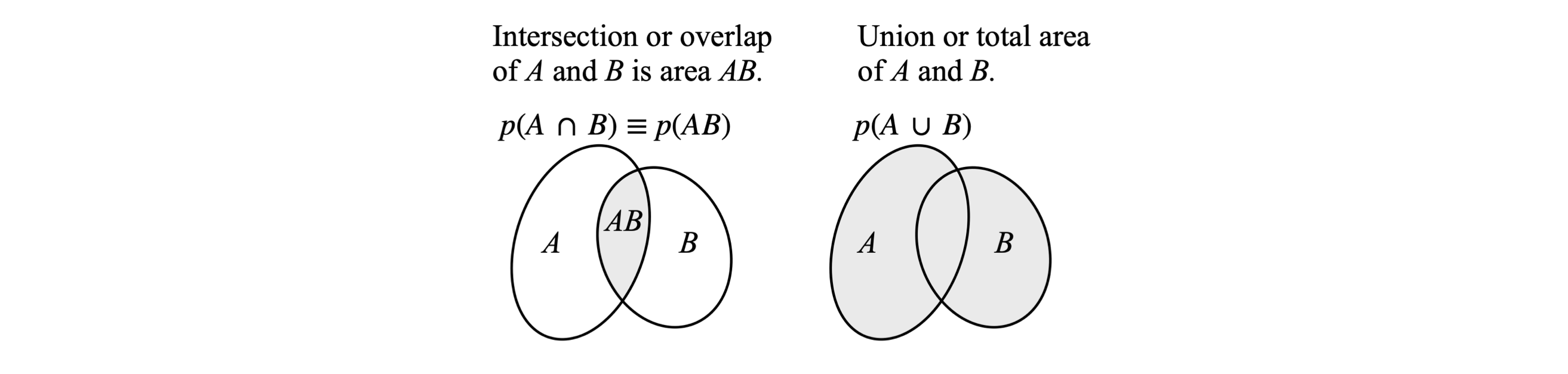
Figure 20. Venn diagrams. Left: A and B are two overlapping ellipses, AB is their overlap and is shaded. The chance of A or B being observed is the intersection of A and B, which is \(p = p(A) + p(B) - p(A, B)\) and is proportional to the total area within the circles less that area overlapped. If A and B do not overlap the events are mutually exclusive and \(p(AB) = 0\). Right: The union of A and B is the chance of belonging to at least one of A and B and is the shaded area.
9.13 Definitions, notation, and some useful formulae#
(i) Definitions. Mutually exclusive vs. independent events.#
A mutually exclusive event is one whose occurrence prevents the other form happening at the same time. Tossing a coin can only produce a head or a tail, if a head is observed the tail is prevented from happening and vice versa, both occurring is prevented.
Independent events mean that one outcome does not influence the other, and so these events cannot be mutually exclusive. Throwing a dice and tossing a coin are independent events, as are tossing two coins, the result of one does not influence that of the other and vice versa.
(a) The probability of an event \(A\) is \(0 \ge p(A) \le 1\).
(b) The certain event \(S\) has a probability of 1; \(p(S)=1\).
(c) The probability of an event \(p(A)\) is the sum of simple events in the sample space.
(d) The word ‘or’ is used in the inclusive sense. Thus, A or B means ‘either A or B, or, both’. The notation \(p(A + B)\), is the probability that either \(A\) or \(B\) or both occurs. The notation \(p(AB)\) is a joint probability and means that both \(A\) and \(B\) occur. In set theory, this is the intersection or overlap of \(A\) and \(B\), and is usually written as \(p(A\cap B)\); figure 20.
(e) If several independent events each of a probabilistic nature occur to produce a successful outcome, then the overall chance of this happening is the product of the probabilities of the individual events, (Product Rule). An independent event is one whose outcome does not influence that for any of the others; \(p(A \& B) = p(A)p(B)\).
(f) If two events \(A\) and \(B\) can occur, their inclusive probability \(p(A + B)\) means that at least one event occurs, which is to be interpreted as event \(A\) or \(B\) occurs. In figure 20 (left) the sample spaces are related as
The area \(n(A)\) and \(n(B)\) is the whole of their respective ellipses, \(n(A + B)\) is the total area less the overlap \(n(AB)\). When divided by the number of arrangements in the sample space these numbers become probabilities. The inclusive probability, either \(A\) or \(B\) or both, is the probability that \(A\) occurs, plus, the chance that \(B\) occurs minus the chance that both occur or
(g) A mutually exclusive event is one whose outcome prevents any others occurring. The two events \(A\) and \(B\), are mutually exclusive if there is no intersection or overlap of \(A\) and \(B\), \(p(AB) = 0\), therefore the probability of the occurrence of at least one out of two possible events is the sum of the individual probabilities, (Addition Rule),
This equation only applies to two events.
(h) The sample space in tossing a coin is heads and tails, (H, T); in tossing a die this is \((1 \cdots 6)\), in one set of playing cards \((1 \cdots 52)\), and so forth. If three coins are used, the sample space contains \(2^3\) elements, HHH, HHT, etc. If \(n_S\) represents the number of arrangements in the whole sample space, \(n_A\) the subset that is the number of ways of arranging events in a successful outcome (call this \(A\)) and \(n_{NA}\) the subset that is not \(A\) then, clearly, \(n_S = n_A + n_{NA}\). The probability of outcome \(A\) is therefore
(i) If \(p\) is the chance that an event occurs, then \(1-p\) is the chance that it will not, (Subtraction Rule),
This is called the complement. On the right of figure 20, the complement of \(p(A\cup B)\) is the area outside the two shaded circles. In the left-hand sketch, the complement of the intersection \(p(A\cap B) \equiv p(AB)\), is all the area not labelled \(AB\) inside the square.
(j) Two objects can be placed into either one or the other or both of two different boxes, hence are distinguishable, then the outcomes are (AB, -), (-, AB), (A, B), (B, A). As each of these is a simple event, the probability of each occurring is 1/4. If the objects are indistinguishable, then there are three arrangements (xx, -), (xx, -), (x, x), but the last may be considered to be two events and in this case would occur with a probability of \(2/4\). However, if we take the three outcomes to be equally likely then the probability of the last is \(1/3\), and this is the case for bosons.
9.14 Independent and exclusive events, sample spaces, and conditional probability#
(i) Chance of observing a head on a coin and a \(6\) on a dice#
If a coin and a die are thrown they are clearly independent events and the chance of observing a head and a \(6\) is \((1/2) \times (1/6)\). This follows from the fundamental principle of counting; if a job is completed in \(n\) ways and another in \(m\) ways then both can be completed in \(n \times m\) ways. For instance, if there are \(6\) types of anions and \(8\) types of cations then \(48\) different salts can be produced.
(ii) Throw two dice to get a given total#
Suppose that two dice are thrown (or the same one twice) and you want to find the chance that the total of their numbers is \(10\). The two dice are independent, the result of one does not influence the other, and the probabilities therefore multiply. As one die can fall in one of six ways, two can fall in \(6 \times 6 = 36\) different ways, (Product Rule). The number \(10\) can be obtained in three different ways, each of which is equally likely to occur: \(6 + 4,\, 4 + 6,\) and \(5 + 5\). The probability of observing \(10\) is therefore \(3/36\). If a sum of \(6\) is sought, then this is produced in the combinations \(1+5,\, 5+1,\, 4+2, \,2+4, \, 1+3\) and would be expected to be observed \(5/36\) times the dice are thrown.
(iii) Cards drawn in succession#
If you want two cards containing the number \(7\) to be drawn in succession from a pack of \(52\) playing cards, what is the chance of this happening if the first card chosen is not replaced in the pack? The chance of the first \(7\) being chosen is \(4/52\) because there are four \(7\)’s in a pack of \(52\) cards. It is now assumed that a \(7\) has been removed and therefore the chance that the second card removed is a \(7\) is \(3/51\) making the chance \((4/51) \times (3/51) = 1/221\) overall and the Product Rule is used. The second choice is \(3/51\) because we have only \(51\) cards left and one \(7\) is assumed to have been removed in our first try. Had we chosen to find the probability that a \(7\) and a \(6\) were to be removed in succession, the chance would be \((4/52) \times (4/51)\).
If instead we wanted to draw either a \(7\) or a \(6\) from the pack, then the probability would be \(4/52 + 4/52\) as these are independent of one another; drawing one card does not depend on the other. Using ‘either or’ usually means that the Addition Rule is used.
(iv) Independent events. Molecular yield#
Independent events can occur in the way molecules react. If a molecule can react to produce two different products A and B with rate constants \(k_A\) and \(k_B\) respectively, the chance of product A being observed is \(p_A = k_A/(k_A + k_B)\) and of B is \(1 - p_A\), which is \(p_B = k_B /(k_A + k_B)\). The sum of both events is 1. In chemistry, probability \(p_A\) is normally called the yield of A and is often expressed as a percentage. If an excited state of a molecule can fluoresce with rate constant \(k_f\) or produce another state such as a triplet by intersystem crossing with rate constant \(k_i\) then the fluorescence yield is \(k_f /(k_f + k_i)\) and the triplet yield \(k_i /(k_f + k_i)\).
(v) Cards drawn but not replaced#
Suppose that two cards are drawn from a pack and the first not replaced, and we want the chance that the second is a \(7\) of diamonds. This question has two answers. If the first card happens to be the \(7\), then the chance of the second being this card is obviously zero. If the first card is not the \(7\) of diamonds, the chance of choosing it a second time is \(1/51\) making the chance \((1/52) \times (1/51)\) overall.
(vi) Throw a die \(n\) time#
Suppose a die is thrown \(n\) times, what will be the chance that a \(3\) appears at least once? Usually when the expression ‘at least once’ is used we use the Subtraction Rule to find the chance that the outcome wanted does not occur. In one throw the \(3\) appears with a chance \(1/6\) and there is a \(5/6\) chance that it does not appear. After \(n\) throws, then the chance is \((5/6)^n\) that the \(3\) does not appear and therefore \(1 - (5/6)^n\) that it appears at least once. For two throws, this is \(11/36\).
This calculation can also be described using inclusive probability. Suppose that there are two outcomes A and B, and at least one outcome is required, then the probability is that of event A, plus event B minus that of both A and B or p = p(A) + p(B) - p(AB). The chance that a \(3\) is thrown, is \(1/6\) on the first throw (outcome A), and again on the second throw is \(1/6\), and the chance of both occurring p(AB) = \(1/36\) making \(1/6 + 1/6 - 1/36 = 11/36\) overall.
9.15 Summary#
If \(n\) and \(m\) are the numbers \(1\) to \(6\) (the sample space) on a die, then the probability of throwing;
(1) any number \(n\) is \(1/6\) and of not throwing any \(n\) is \(1-1/6\).
(2) either \(n\) or \(m\) is \(1/6+1/6 = 1/3\). (Addition Rule)
(3) the same \(n\) twice in two throws is \((1/6)(1/6)\). (Product Rule)
(4) any number twice in two throws is \(6\cdot (1/36)=1/6\). You don’t care what the first number is just that the second matches it. The table shows all the possible outcomes (sample space) and is often a convenient way of working out probabilities. The \(6\) double numbers are outlined.
(5) \(n\) at least once in two throws is \(1 - (5/6)^2 = 11/36\). (Subtraction Rule)
(6) \(n\) exactly once in two throws is the chance on the first throw of getting the number \(n\) with the first dice but not the second, and the other way round on the second throw which is \(\displaystyle\frac{1}{6}\cdot\frac{5}{6}+\frac{5}{6}\cdot\frac{1}{6}\). The chance of not getting \(n\) on either throw is \((5/6)^2\). These results can be seen in the table above.
(vii) Same birthdays#
To illustrate explicitly the use of a sample space, consider the problem of calculating whether at least two people from a group of \(25\) people have the same birthday (see Goldberg 1986, p. 53). First, to simplify the calculation it is necessary to ignore leap years, and then to assume that there are no twins in the group and that births occur with equal probability throughout the year. None of these may be true in a real sample of people, but we will assume that they are.
The sample space is defined as the total number of arrangements \(n_S = n_A + n_{NA}\) split into those in the group we want to determine \(n_A\), and those that we do not, \(n_{NA}\). The sample space is huge, \(n_s = 365^{25}\), because this is the number of ways that the birthdays can be arranged. Let \(n_A\) be the number of arrangements where at least two people have the same birthday and \(n_{NA}\) the number of those with different birthdays, then \(n_{NA}\) is the number of ways of selecting \(25\) different days from \(365\).
The first birthday can be chosen in \(365\) ways, the second in \(365 - 1\) and so forth down to \(365 - (25 - 1)\) ways. This makes
which is the permutation \(P(365, 25) = 365!/(365 - 25)!\).
The number of different ways that \(25\) people can be selected is therefore
The probability that at least two people have the same birthday is
if we assume that each of the \(365^{25}\) outcomes is equally likely. The result is
It is surprising that in such a small group the chance of two or more people having the same birthday is so large. When the number of people is small then the chance of any two having the same birthday approaches zero, as the number increases so must the chance of any two having the same birthday. In fact above \(60\) persons the chance is almost \(100\)%.
The problem can be tackled in another way. The chance that the first person has a birthday on any day is obviously \(365/365\), the second person now only has 364 days to be born on so their chance is \(364/365\), and so on to the last person with chance \(341/365\). The complement of the product of all these numbers gives the answer above.
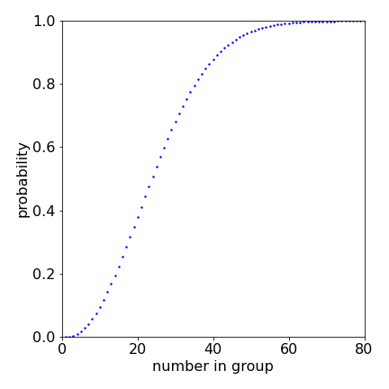
figure 20a. Probability that two people in a group of \(n_A\) have the same birthday.
This problem can be stated in a different way. If you know \(n\) peoples birthdays is it more likely or not of two of them being on the same day and month (Rouse Ball & Coxeter, 1987). If everyone has a different birthday, so that there is a random selection of \(n\) days out of \(365\), the total number of selections is \(365^n\). As each day should only be counted once the number of selections becomes \(365\cdot364\cdots (365-n+1)\), thus the probability is
Let the occurrence be just as likely as not then the probability is \(1/2\),
and we can evaluate this by rearranging. The first three terms are \(\displaystyle \frac{365}{365}\frac{364}{365}\frac{363}{365} = \frac{365-1}{365}\frac{365-2}{365}=\left(1-\frac{1}{365}\right)\left(1-\frac{2}{365}\right)\) and so the product is
taking logs of both sides and using the log expansion as each term is small ( \(\ln(1+x)=x )\) produces
which is \(\displaystyle 1+2+\cdots n-1=365\ln(2)\) and the summation is equal to \(n(n-1)/2\) making the result
from which \(n= 23\) to the nearest whole number. You can see from the plot above that this value of \(n\) is \(1/2\).
(viii) Conditional probability. Throwing coins#
Sometimes conditional probabilities are required; for example, tossing three coins and deciding what is the chance that the outcome is at least two tails (outcome A) and knowing that the first coin to fall is a head (outcome B). Tossing three coins can only produce the patterns
\(\qquad\qquad\) HHH, HHT, HTH, HTT, THH, THT, TTH, TTT
and each has a chance of \(1/8\) of being produced in three throws. The first outcome (A) is the chance of having at least two tails and by direct counting this is \(p(A) = 4/8\). The chance of having a head as the first coin is \(p(B) = 4/8\). The chance that both conditions apply, is calculated \(p(A, B) = 1/8\) by inspecting the sequence of coins. The conditional probability \(p(A | B)\), is the chance that both conditions apply divided by the chance that condition B applies, and this is
which is \(1/4\). This means that the added knowledge that the first coin to fall must be a head, has reduced the odds of obtaining two tails, which is not unexpected since insisting on a head as the first coin reduces the choices available. The equation is ‘symmetrical’ and can be rearranged to
(ix) Passwords#
Finally in this section consider a hacker using a computer to guess what your password is. Of course this could happen by random chance happen on the first try but the chance is small if the password is made up of random characters, letters and numbers. However, the hacker can easily try \(10^8\) times with a computer so probabilities become a consideration
Suppose that the requirements are very low, such that the password must have four letters, two of which are capitals and four numbers. As there are \(26\) letters in our alphabet and ten numbers (\(0\to 9\)) the total number of passwords is
\(N= 26^2\cdot26^2\cdot10^4=4,569,760,000\)
and so the chance of guessing correctly is \(1/N\) which is quite small. Now the chance of not guessing correctly is \(1-1/N\) and to do so \(10^8\) times is \((1-1/N)^{10^8}\). Therefore the chance of guessing correctly is the complement of this which is
and is \(0.021\) or \(2.1\)% which you might think is a good enough risk for you but is rather high if many millions of passwords are being challenged. If the hacker tried \(10^{10}\) times then the chance of guessing correctly is \(87\)%, very high indeed.
Adding one or two non-alphabetical characters such as space, dash, question mark etc. really helps as would more random numbers and letters. Thus if the password contains \(15\) characters for example \(8\) letters, \(4\) numbers and \(3\) non-alphabetical characters (there are at least \(30\)) the total number of possibilities is \(N =26^8\cdot 10^4 \cdot 30^3 \approx 5\cdot 10^{19}\) and the chance of guessing after the huge, and possibly impractical, number of \(10^{18}\) guesses is still effectively zero.
9.16 The Binomial distribution (See also chapter 12.3)#
The binomial distribution is used when an experiment has two outcomes, often labelled as success or failure. A ligand binding to a molecule can be considered a success and therefore not binding, a failure. If the molecule is a protein then the terms ‘on’ and ‘off’ or ‘bound’ and ‘unbound’ are often used to describing binding and not binding.
Success may be considered to be a head when tossing a coin, and so a tail is a failure, or throwing a \(2\) when tossing a die and any other number a failure and so forth. In a trial let the chance of success be called \(p\) and of failure, therefore, \(1-p=q\) as the total chance must be unity. When there are \(n\) trials (coins for example) the chance of achieving \(n\) successes is \(p^n\) and thus the chance of failure \((1-p)^n\). If we want \(m\) successes (say heads) and therefore accompanied by \((m-n)\) failures (tails) the sequence of heads and tails could be \(hhthtthh\cdots\) with probability \(P=ppqpqqpp\cdots\) which with \(m\) successes is for this specific sequence the probability is
where \(n\) and \(m\) must be integers, we cannot have, for example, 3.5 coins or 4.1 successes.
A binomial distribution thus requires three conditions to be met,
a fixed number of trials \(n\),
a constant chance of success \(p\) and
each test independent of all others.
(i) Multiplicity or Binomial Coefficient W#
Usually we are not interested in a specific sequence but in sequences that have the same number \(m\) of successes and so we need to find the number of these. To do this we imagine filling \(n\) boxes with a head or tail coin where each choice in independent of all others. There are \(n\) ways of choosing the first box, and \((n-1)\) the second as one is already filled, \((n-2)\) the third and so on making \(n!\) ways in total.
However, we want \(m\) of these coins to be heads (success), and so \((n-m)\) must be a failure. The \(m\) successes and \((n-m)\) failures can occur in any order during the \(n\) trials as each trial is independent and is either a success or a failure. However, there are many ways in which \(m\) successes can be achieved in \(n\) trials and we are only interested in the total number of successes not in what order they occurred. The number \(n!\) clearly over counts the number of possibilities and so we have to reduce this number by \(m!\) ways of obtaining a success and by \((n-m)!\) for failures. The number of ways that success can be achieved is therefore
and this is also the number of Combinations \(\displaystyle C^n_m=\binom{n}m\). This can be explained in another way. Since ‘heads’ can be distributed in \(m!\) ways and similarly ‘tails’ in \((n-m)!\) ways the total number \(n!\) must be divided by \(m!(n-m)!\) ways. As the factorials are often large and difficult to calculate Stirling’s formula provides an accurate way of doing this.
(ii) Binomial distribution#
The probability of achieving \(m\) successes in any order from \(n\) trials is the multiplicity \(W\) multiplied by the probability \( p^m(1-p)^{n-m}\) which is
and is called the Binomial Distribution because the Binomial expansion is
and the coefficients in this distribution are the multiplicity \(W\). The probability \(p\) is not generally \(1/2\) and this is like throwing a biased coin, which favours either heads or tails.
This distribution is normalized \(\sum_{m=0}^n B(n,m,p)=1\) because \(p+q=1\) and so \((p+q)^n =1\). The average value of the distribution is at \(m\) equal to \(\mu=np\) which gives its maximum value when \(\mu\) is substituted for \(m\). The variance is \(\sigma^2= np(1-p)\).
The binomial distribution, and the Gaussian and Poisson distributions which are derived from it, are examined in more detail in Chapter 13 where descriptive statistics are discussed.
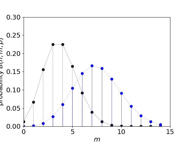
Figure 20b. The Binomial distribution with \(n=15, p=1/4\), left with black dots and \(n=30, p=1/4\), right, blue dots. The distribution is shown only at discrete points \(m\) with a line joining these only to guide the eye.
(ii) Binomial Expansion#
The binomial expansion can be worked out by choosing items from boxes. If a box contains a mixture of a large number \(w\) of white balls and \(b\) black ones, and if one ball is chosen, the chance of choosing a white ball is \(p = w/(w + b)\) and correspondingly a black one \(q = b/(w + b) = 1 - p\).
If there are two boxes, \(n=2\), the probabilities are distributed in the same manner as tossing two coins. The coins land as HH, HT, TH, TT and each has a \(50\)% chance of being H or T, therefore the probabilities are
because HT is the same as TH. Choosing white and black balls from two boxes has the equivalent probability \(p^2,\; 2pq,\; q^2\) or \((p+q)^2\).
Continuing for more boxes and expanding shows that the general form is \((p+q)^n\). The symmetrical nature of the series for binomial expansion can be seen by working out some terms for example,
where the powers of \(p\) and \(q\) always add up to the same total \(n\) and the factorials are symmetrical and in this case have the values \(1,4,6,4,1\) which form part of Pascal’s triangle and which can be used to work out values if needed. The values in this triangle are the sum of the two immediately right and left above. The first row must be labelled zero.
The coefficients are the multiplicities \(W\) given above and the sum of these is
The sum is found by supposing that we select balls from a \(1:1\) mixture of a huge number of two types of them then the chance of selecting, say, a red or white one must always be \(1/2\). The probability of selecting two white balls in succession is \((1/2)^2 \) and of selecting \(20\) in succession the minute chance \((1/2)^{20}\) and so on. The chance of selecting any given sequence of length \(n\) is just \((1/2)^n\). The number of configurations is simply the inverse of this, thus the sum of the coefficients is \(2^n\), i.e. \(2^3=1+3+3+1\) as can be checked in the Pascal triangle.
(iii) Combinations#
To see how the combination terms represent the probability think of the chance of selecting \(m\) objects out of \(n\), the total number of them. Suppose that the first of these chosen is of type \(A\) and has a probability of being chosen (or measured) as \(p\). The second chosen of type \(A\) then has a probability \(p^2\) and if all chosen are of type \(A\) the probability is \(p^m\). If exactly \(m\) are of type \(A\) then \(n-m\) are of another type and this probability is \((1-p)^{n-m}\), thus out of our particular choice of \(m\) objects the probability that they are all of type \(A\) is \(p^m(1-p)^{n-m}\). As this choice is not the only one, because the first \(m\) objects can clearly be chosen in another way, in fact \(n\) different ways for the first item and \(n-1\) for the second and so on leading to \(n-m+1\) in total. The product of these ways of choosing is
However, this number is too large because it counts choices that differ only in the order of choosing the \(m\) objects (\(m_1m_2\cdots\) is the same as \(m_2m_1\cdots\) ) and so should be divided by the number of permutations of these \(m\) which is \(m!\) making the final multiplier \(\displaystyle \frac{n!}{m!(n-m)!}\), which is the term in equation 25a.
(iv) Chance of drawing red cards from many packs#
In calculating the probabilities, the values of \(p\) have to be found from the problem at hand. For instance, to find the chance that no red cards are drawn in a single attempt from each of seven packs of cards, we need to know that half the cards are red. As \(p = 1/2\) this chance is
The chance of picking four red cards from the same number of packs is
and of picking four picture cards (12 in each pack) out of five packs of \(52\) cards each, is
The chance of obtaining an even number of aces from six packs of cards, is \(313201/4826809 \approx 0.065\) and is the sum of choosing 2, 4 and 6 aces, each with a chance \(p = 4/52\).
(v) Chance of getting the same number in many throws of a die.#
What is the chance that after \(12\) tosses of a die the number \(3\) will appear twice or less. The chance of getting a \(3\) (or any number) in any throw is, of course, \(1/6\). The probability that a \(3\) will not appear is when \(m=0\) in eqn 25a or,
Similarly, the chance that the number \(3\) will be seen once is
and appear twice is \(B(12,2,1/6)=0.296\) and the probability of \(3\) appearing twice or less is the sum of these and is \(0.874\). This fraction goes down as the number of trials \(n\) increases, and this is because the total probability must be unity and as the number of trials increases the number of other possibilities increases making the chance of \(0+1+2\) smaller. The calculation is shown below.
# Calculation of probability by Binomial Distribution

n, m, p = symbols('n, m, p')
n = 12
p = 1/6
prob = lambda n,m,p: factorial(n)/(factorial(m)*factorial(n-m))*(p)**m*(1-p)**(n-m)
print('{:s} '.format('   m  B(n,m,p)    sum' ) )
s = 0
for m in range(n):
    s = s + prob(n,m,p)
    print('{:4d} {:8.6e} {:8.6f}'.format( m, prob(n,m,p), s ) )
   m  B(n,m,p)    sum
   0 1.121567e-1 0.112157
   1 2.691760e-1 0.381333
   2 2.960936e-1 0.677426
   3 1.973957e-1 0.874822
   4 8.882807e-2 0.963650
   5 2.842498e-2 0.992075
   6 6.632496e-3 0.998707
   7 1.136999e-3 0.999844
   8 1.421249e-4 0.999987
   9 1.263333e-5 0.999999
  10 7.579995e-7 1.000000
  11 2.756362e-8 1.000000
(vi) Most probable number of tails in many throws of a coin#
A coin is tossed \(12\) times, what is the most probable number of tails and what is the most probable number? THe probability of obtaining a tail on any toss is found using eqn 25a with \(n=12, p=1/2\) leaving \(m\) to be determined, viz
The simplest approach is to use the computer to calculate the values. SymPy has a built in factorial (and binomial) function. From the results the most probable number of tails is six with a probability of \(0.225\). In fact the most probable is always \(n/2\) as the distribution is symmetrical.
9.17 Chance of getting \(4\) heads in \(12\) coin flips#
In this case imagine that the coins are labelled H or T and there are many possible lists of the coins such as HTHHTTHTTHH among which are those that have only \(3\) heads. The strategy is therefore to find the number of lists and so the chance of having any list whatever its composition, and then the chance that any one of these has only \(3\) heads.
The coin can only be either H or T therefore there are only two choices to make each time and assuming fair coins means that each flip made to extend the list is independent of all previous ones making a total of \(2^{12}=4096\) lists to choose from. The total probability of all events must always be \(1\), therefore the probability of any one list such as HHHHHHHHHHHH or HTHHTTHTTHH is \(\displaystyle \frac{1}{4096}\). Perhaps this seems strange. If you do a fair lottery any combination, even one will all the numbers the same, should have an equal, but minute, chance of being chosen.
Now the chance of choosing to get \(4\) events out of \(12\) is needed. This is found using the binomial distribution
and so the chance of throwing a sequence of \(12\) coins with \(4\) heads is \(495 /4096\). Of course, equation 25a could be used directly with \(p=1/2, q=1-p=1/2, n=12, m=4\) or
9.18 Similar random digits#
What is the probability of finding at least \(m=100\) similar digits such as \(0\) or \(3\) etc., in \(n=1000\) random digits. There are only \(10\) types of digits, so using the binomial distribution the probability for \(m\) similar digits gives (eqn. 25a)
but this has to be summed from \(m\to n\) to find at least \(m\) so that the probability becomes
As \(m\) increases this probability falls rapidly. The calculation is shown below using SymPy. The factorials are extremely large, and SymPy has a factorial function that will calculate these, as shown below, and there is also a \(binom(n,m)\) function that calculates the binomial coefficient directly. The same result can checked by repeatedly making a random list of \(n\) digits and checking how many are equal to or larger than \(m\).
n, m, p = symbols('n, m, p')
n = 1000
m = 100
p = 1/10
prob = lambda n,m,p: factorial(n)/(factorial(m)*factorial(n-m))*(p)**m*(1-p)**(n-m)
print(prob(12,1,1/6))
s = 0
for i in range(m,n,1):
    s = s + prob(n,i,p)
print('{:s}{:6.3g}'.format('probability B =', s) )
0.269175971483076
probability B = 0.515
9.19 How many fragments are there in a well in a 96 well plate?#
Labelled DNA fragments are randomly distributed into a \(N = 96\) well plate for fluorescence analysis. There are \(n=100\) fragments, what is the chance of having more that one fragment in a well?
Using the Binomial distribution the probability of being in a well (a positive result) is \(p=1/96\), therefore \(B(n=100, m, p=1/96)\), gives the chance of \(m\) fragments in a well. The average number is \(\mu=n/N\). This calculation is just the same as putting coins into boxes as we can consider each well as a box. Calculating the fraction with none \(m=0\) and one present \(m=1\) and subtracting these from unity gives the probability of more than one fragment in a well. The calculation for \(m\) present is
which is \(35.1\)% empty wells and \(36.9\)% with one fragment and therefore \(28\)% have more than one fragment.
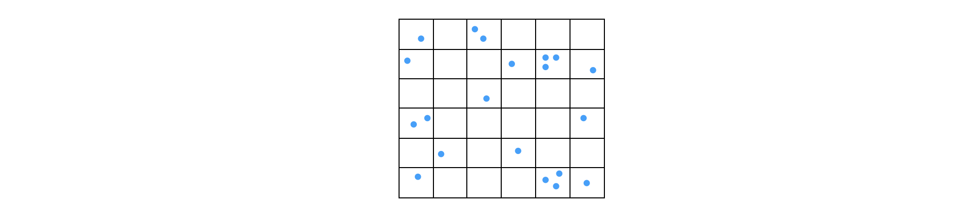
Fig20c. Distribution of fragments in a \(36\) well plate. The wells are equivalent to boxes into which particles (or coins etc.) are placed when working out the probabilities.
9.20 Red shifted tryptophan fluorescence#
The fluorescence of tryptophan residues in several types of proteins shows variations in emission wavelength over a range of several nanometres around \(340\) nm. Most shifts, but not all, are to the red of tryptophan in solution. It is suggested that this red shift is due to the presence of electric fields present in the proteins that are caused by nearby residues. The effect might of course just be random, however, only \(3\) in \(19\) different types of protein have blue shifts so its seems that a random effect is unlikely. As a check the binomial theorem can easily be used. There are two choices, red shift or blue shift and so the chance of a blue shift is
which clearly shows that this is unlikely to be a random effect.
9.21 Isotopes#
Consider finding the chance that at least one atom in C\(_{60}\) is a \(^{13}\)C. This isotope is only present at \(1.109\)% and \(^{12}\)C as \(98.89\)% because carbon only has two stable isotopes. If we find the chance that no \(^{13}\)C is present then one minus this number is the chance that at least one is present. Of course, it is also possible to find the chance that \(1,2,\cdots\) only are present.
There are \(60\) atoms therefore out of \(n = 60\) only \(m\) will be \(^{13}\)C and so \((n-m)\) \(^{12}\)C. We shall choose \(m = 0\), i.e. the ‘success’ that none are present. The probability \(q = 0.01109\) and the calculation that there is no \(^{13}\)C is present sets \(m=0\), i.e \(B(60,\,0,\,0.01109)\). To calculate this may seem odd but \(1-B\) is the chance that at least one atom is present and is what is sought.
which means that there is \(\approx 49\)% chance that at least one \(^{13}\)C is present in each C\(_{60}\) molecule, which is a good outcome if one is doing a \(^{13}\)C NMR experiment.
A similar calculation is that to find the chance of having one \(^{13}\)C and one \(^{15}\)N in a molecule with 10 carbons and 2 nitrogens. The probabilities of having both multiply together the chance of each singly.
Rather than use the formula we work out step by step. The probability of one \(^{13}\)C is \(0.01109\) so the chance of not having one is \((1-0.01109)^9\). The probability of the first one being \(^{13}\)C is \(0.01109(1-0.01109)^9\), however, this carbon could be in any position so we multiply by \(10\) to give \(10\cdot 0.01109(1-0.01109)^9 = 0.10\) which is \(B(9,1,q)\). The calculation for the N atom gives \(0.069\) so the joint probability is \(0.0069\).
9.22 Chromatography#
The shape of a peak as a result of measuring some property of molecules in the mobile phase eluted in a chromatography column will calculated and to do this the column is split into a series of \(N\) theoretical plates just as is done for a distillation column. In each theoretical plate there is equilibrium between the mobile and the stationary phase, but not between one plate and its neighbour because the mobile phase flows through the column. The solid or stationary phase consists of the packing material in the column and onto which the solute adsorbs and then desorbs back into the mobile phase at a later time. The number of plates is large, typically several hundred to a few thousand per metre of column. This is a model based just on probabilities and ignores any of the kinetics of forming and being released from a surface or any molecular properties.
To calculate the movement down the column we suppose that movement happens in a series of steps \(n\) and because the mobile phase flows through the column \(n\) can be larger than the number of theoretical plates. Initially \(m_0\) moles of solute injected into the column and equilibrium is formed (mobile to solid phase) in the first plate producing \(m_0p\) in the mobile phase and \((1-p)m_0\) in the stationary phase. Next, the mobile phase with its amount \(m_0p\) solute at plate 0 passes this to plate 1 (initially empty) and plate 0 and 1 reach equilibrium. Note that just after moving to plate 1, the mobile phase in plate 0 has has zero solute until this equilibrates with the solid phase. At step two the amount in the mobile phase in plate 1 moves to plate 2, and plate 2 equilibrates, and the amount in the mobile phase in plate 0 also moves to plate 1 and equilibrates again. The process repeats as molecules move down the column.
You can understand that as some molecules are retained at each step on the stationary phase the injected material initially in plate 0 spreads out among the plates as the mobile phase moves along the column. The profile observed at the end of the column by the detector will therefore have a certain rising and falling shape depending on just how long the molecules are retained at each plate, i.e. depending on the partition constant between stationary and mobile phases vs. how fast the flow rate is. As the amount injected into the column is fixed, the broader the detected profile is the less is its intensity. Clearly what is aimed for is an intense narrow profile so that many species can be identified at once depending on their differing partition constants.
The equilibration partitions the amount in the mobile and solid phase as \(p:(1-p)\). The calculation for the fist step is that \(m_0p\) is partitioned into the mobile phase and therefore \(m_0 - m_0p = m_0(1-p)\) adsorbed onto the stationary phase. In the next step the mobile phase moves to the next empty plate and \(m_0p\) is partitioned between phases meaning that at equilibrium \(m_p^2\) is in the mobile and \(m_0p(1-p)\) in the stationary phase. The amount \(m_0p^2\) is transferred to the third plate and equilibrated, and \(m_0p(1-p)\) from the first plate moves to the second and equilibrates. The table shows the scheme. Note the symmetry in the terms at each state, and that the constants follow those of the binomial distribution and Pascal’s triangle, 1, 11, 121, 1331.
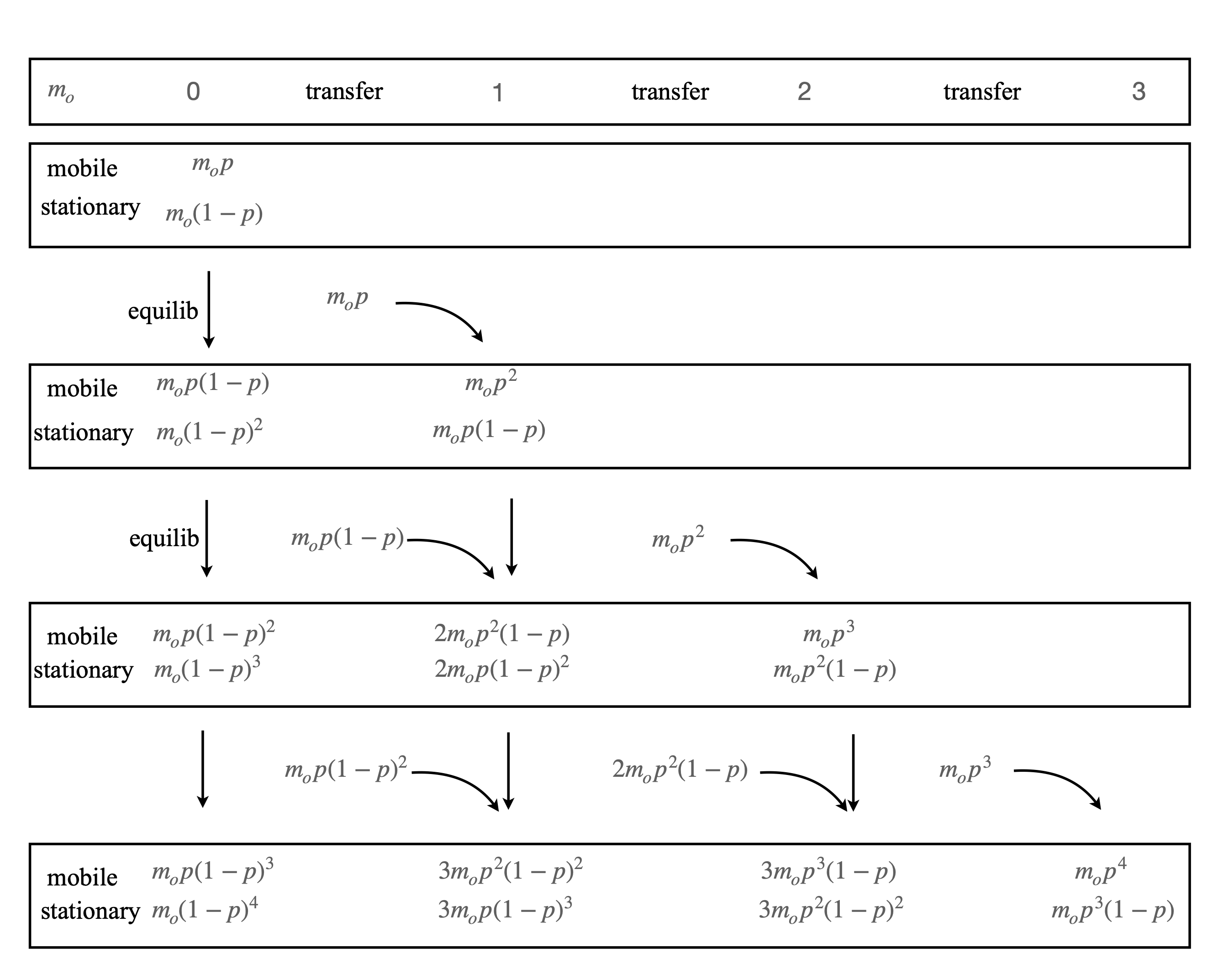
Table 1: Progress down the column and the equilibrium amounts of solute at each stage with plates, \(0,1,2,3\). The vertical lines indicate equilibration, the curved ones transfer.
The total amount at each plate is the sum of the mobile and stationary parts, for example from the last row in the table the totals are,
Repeating the process produces the binomial distribution and at the \(r^{th}\) plate after \(n\) steps, which means a volume \(nV_m/N\) of mobile phase has passed through the column \(V_m\) being the total mobile volume of the column, the total amount is
which is the Binomial distribution and \(m_r/m_0\) can be interpreted as the ‘probability that the molecule will have achieved \(r\) successes in \(n\) tries’. The molecule is most likely to be found at the \(np^{th}\) plate which is the mean value of the distribution.
To be of any use the parameter \(p\) has to be related to the properties of the column, in particular to the partition constant \(K\). If \(V_s\) and \(V_m\) are the total volumes of the stationary and mobile phases in the column respectively, then each plate has volume \((V_s+V_m)/N\). The equilibrium in each plate is found from the partition between mobile and stationary phases, and we have used \(p\) as the fraction of solute in the mobile phase and hence \((1-p)\) is in the stationary phase. The partition constant \(K\) is therefore the ratio of the amount of the solute in stationary to that in the mobile phase or
from which
Normally, we expect the stationary phase to be chosen to have a large value \(K\gg 1\) for the type of molecules being separated, therefore \(p\) is very small, but has to be different for different molecules for separation to be achieved. As \(p\) is small binomial distribution can be approximated with the Poisson one. (This calculation is shown in the next section). The amount at the \(r^{th}\) plate becomes
If we measure the amount in the eluted solution, i.e mobile phase, at the last but one plate (\(N-1\)) then the total amount is split as \(p:1-p\) between the mobile and stationary phase, the probability of the \(n^{th}\) volume fraction \(V_m/N\) measured is thus
which is the probability that a molecule will be eluted. This is the Poisson distribution multiplied by \(p\), it still has the shape of the Poisson distribution which for large average value is approximately a ‘bell shaped’ curve. In chapter 4.8 the width of the eluted curve, which needs a knowledge of integration, is examined. (This example is based on one by C. Perrin, ‘Mathematics for Chemists’ publ. Wiley 1970).
9.23 Large numbers and most probable state.#
An alternative way of forming the binomial coefficient \(\displaystyle \frac{n!}{m!(n-m)!}\) in equation 25a is to consider many of two different types of atoms, e.g. He and Ne, or types of snooker balls, e.g. red and white which gives a reasonable analogy as He and Ne have no strong interactions between then when not in contact and neither do billiard balls. Suppose that we place the balls into a jar so that red and white layers are apparent. Next by shaking the jar this arrangement is lost and a irregular looking one is formed. In fact if shaking is continued the ordered layers are almost never going to be seen again. This means that the ordered starting point is just one possibility of a truly vast number of others and returning to the original arrangement is highly unlikely which means that the probability of this is extremely small.
Suppose that there are \(n=100\) similar balls, \(50\) each red and white and that they are numbered, \(1,2\cdots 100\) irrespective of colour, and they are randomly placed to fill \(100\) positions. In placing the first ball there are \(100\) choices, the second can go in any of the \(99\) empty places so that in positioning the first two we have had \(100\times 99 = 9900\) choices. Continuing likewise produces \(100\times 99\times 98\) for the third choice and so on until the last ball is in position making the total number of choices the permutation
and each of these is equally likely to occur. If the balls are not numbered but remain coloured, and hence distinguishable, there will be a smaller number of distinguishable arrangements, which is the number of ways of selecting groups \(m\), and this will be smaller than \(n!\) because exchanging any two red balls for any two white ones makes no difference (See also section 9.2). We want to split the balls into 2 groups with, in this case, 50 balls in each but we are not concerned with the order in which they are put into each group. There are \(50!\) ways of putting the first \(50\) white balls into the first half. Next, the number of ways of selecting the \(m\) groups multiplied by the number of permutation in the first and multiplied by the number of permutations in the second group gives the total possible number of permutations. Therefore \(m\times 50!\times 50!=100!\) ways and so the number of distinguishable arrangements \(m\) is the combination,
Evaluating the factorials can be tricky for large numbers and care is needed when computing them, for example \(100! \approx 9.3\cdot 10^{157}\) and larger factorials for relatively small numbers, e.g. 200, can easily exceed the floating point capabilities of a computer. For numbers greater than about \(20\) the Stirling approximation is very good. There are several forms of this but the most common is written as
producing \(m\approx 1\cdot 10^{29}\). This means that the balls must be shaken on average of \(10^{29}\) times before a particular arrangement of the balls is found. At one per second this would take \(\approx 10^{21}\) years, compared to the age of the universe \(1.38\cdot 10^{10}\) years; this is a long, long time even for a small number of particles. The chance of recovering the initial arrangement of layers of white and red balls is effectively zero.
Evaluating \(m\) via the accurate Sterling approximation (above left) and when there are an equal number of balls or molecules produces
for \(n_0\) in total. Thus for half a mole each of He and Ne, \(n_0=6\cdot 10^{23}\) so that the number of configurations is so vast it is impossible to comprehend; \(m=2^{6\cdot 10^{23}}\). This vast number is why it has never been observed, and never will be, that the atoms or molecules of a gas are found in just one part of a bottle, i.e. a vacuum will never spontaneously form in a room . However, if the number of atoms is small, say 10, it may be possible to observe behaviour never seen with larger numbers. Such ‘single molecule’ experiments are now quite common. As will be calculate later, 9.24(i), the chance that the gas will fill only \(99\)% of any volume and not \(100\)% is also vanishingly small.
The probability of observing exactly \(50\)% is
which tends to zero as \(n_0\to \infty\) which is not what we would expect. However, ‘exactly’ is a very restrictive condition and if the distribution of probabilities with different ratios is calculated, as is done next, we find that the \(50\)% probability is always greater than any other and that the probability is sharply peaked at \(50\)% chance.
So far we have considered just a \(50:50\) ratio but of course we need not have chosen equal numbers of red and white balls, the argument is quite general and in doing that we arrive at the general binomial coefficient rather than just a specific term. As other possibilities arise, say \(49\) white \(51\) red producing \(\displaystyle 100!/(49!51!)\) and so on the number of configurations increases and the total for all cases is
which is proved in relation to the Pascal triangle above. When \(n=100,\; m=2^n= 1.26\cdot 10^{30}\) roughly 12 times larger than \(100!/(50!)^2\).
The probability of obtaining a ratio with a number \(k\) of one type of ball (or molecule) out of a total of \(n\) is
This distribution is a maximum when \(k=n/2\). This can be seen with a straightforward argument. The factorial terms are symmetric, \(k!(n-k)!=(n-k)!k!\) and always positive. When \(k=0\) or \(k=n\) the probability is very small tending to zero; i.e \(1/2^n\) is small so there must be a maximum somewhere in the range \(0\to n\). The symmetric nature ensures that this will be at \(k = n/2\). This can also be determined by differentiation. It is not possible to differentiate a factorial, as \(n\) and \(k\) are discrete, but replacing \(n!\) and \(k!\) with the Sterling approximation \((n!=n^ne^n)\) and setting the derivative in \(k\) to zero allows the maximum to be found, viz.,
and the maximum when \(d\ln(W)/dk=0\) is at \(k=n/2\).
The second feature of this probability distribution is that it becomes extremely narrow as \(n\) increases. This is shown in the figure which shows the normalised probability \(p/p_{max}\) vs \(k/n\) which is a fraction between \(0\) to \(1\). At large \(n\) the distribution becomes so narrow, or peaked at \(n/2\), that almost all the probability is described by that at \(n/2\), i.e. this value is so great compared to others that \(p_{max}\) is in effect greater than all others combined.
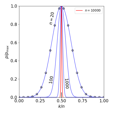
Figure 20d. The peak normalised probability function \(\displaystyle p=\frac{n!}{k!(n-k)!}\frac{1}{2^n}\) vs \(k/n\) for different \(n\). The the data only exists for integer values as shown as circles for \(n=20\), at larger \(n\) a line is drawn as the points become too congested. The curve for \(n=10000\) is in red. At large \(n\) the distribution becomes very narrow and the maximum value at \(n/2\) is greater than all others combined and the distribution can be approximated by its maximum value.
9.24 Entropy#
Returning to the example of using coloured balls and starting with ordered layers, on shaking these balls became mixed up and this is a little like two gases diffusing into one another, however, we supposed that there were \(100\) balls and \(100\) slots to put them into each with the same probability. In reality, in a gas the atoms/molecules (particles) themselves occupy virtually no volume compared to the volume occupied by the gas, thus the number of spaces available is vastly more than the number of particles. We divide the space occupied up into \(w\) minute cells which is a number far greater than the number of particles \(n\). The total number of configurations is found using the familiar equation,
Using the Sterling formula and simplifying gives
Because \(n/w \ll 1\) the log can be rearranged to
and then approximating as \(\ln(1-n/w) = -n/w\) can be done without any significant error to give
Suppose that the volume the gas is irreversibly expanded from \(V_1 \to V_2\) and define \(r = V_2/V_1\), therefore the number of spaces/cells \(w\) changes as \(w \to rw\). The ratio of the number of configurations in the final to initial volume is found using the last equation again and is
meaning that
We come back to this after a short diversion.
(i) Improbability of suddenly finding a vacuum#
A gas always fills the volume available to reach its equilibrium state. At equilibrium the entropy is maximised. To see how improbable it is that a gas would fill just \(99\)% of the volume imagine that there are \(10^{24}\) molecules, just over a mole, and that the other \(1\)% of the volume is empty. The gas is now in a lower entropy non-equilibrium state. Using the last result \(m_2/m_1 = (V_2/V_1)^n\), which is the number of microstates \(m_2\) in volume 2 (\(V_2=0.99\)), divided by those in volume 1 (\(V_1=1\)), the probability is
which is utterly minute and hard to comprehend. Suppose that \(10^{12}\) observations could be made each second to see if a void appeared, this would mean taking \(3\cdot 10^{19}\) /year and if this continued for the age of the universe (\(10^{10})\) years would make \(\approx 10^{29}\) observations. However, this would not be of any help at all as it represents only \(4\cdot 10^{\large{-4\cdot 10^{21} -29}}\) of the total, an utterly insignificant amount. Just to be clear \(10^{10^{21}}\) is \(1\) followed by
The minute chance of observing even a small void illustrates that the equilibrium state is overwhelmingly probable, in fact far greater than all other possible states combined.
(ii) Entropy change on expansion#
To connect eqn. 25d with the entropy, this is derived from classical thermodynamics. The change in entropy \(S_2 - S_1\) upon expanding an ideal gas irreversibly from volume \(V_1\to V_2\) with no addition of heat and without doing work is calculated using
In Thermodynamics entropy is always calculated using \(\int dQ_{rev}/T\) so a reversible pathway always has to be found even if it is not realisable experimentally. As no heat or work is exchanged with the surroundings the change in internal energy is zero (for a perfect gas), \(\Delta U = 0\) and the temperature \(T\) is unchanged. To find a reversible path suppose that the gas is in a cylinder with a movable piston connected to a heat reservoir at constant temperature \(T\) and this arrangement allows the change from state \(T_1V_1\to T_2V_2\). As the piston moves reversibly the pressure on either side of it is always the same. Using the first law with \(\Delta U = 0\) and \(dW_{rev}= -pdV\) gives
Integrating gives the entropy change on expansion,
Notice that the entropy change does not depend of the properties of the gas just its volume or mole fraction since \(pV=nRT\) and assuming one mole in total. From our previous equation (25d) it follows that
The ratio \(R/n\) has a special meaning when \(n\) is the Avogadro number when it becomes the Boltzmann constant \(k_B\). It is normal to choose some reference state for the entropy, just as we choose (mean) sea level as the zero of height on a map, thus the entropy is defined as
which is the form of equation first derived by Boltzmann. The most natural state to choose as the zero of entropy is a pure substance, e.g. a perfect crystal at 0 K, where the substance is in perfect arrangement so that \(m = 1\) and \(S_0 = 0\). Glasses and solid solutions will not have zero entropy at 0 K neither do some molecules such as CO because of orientational variation, i.e. energetically orientation CO-CO is little different to CO-OC.
We have found that the distribution that \(m\) represents is very sharply peaked at its maximum, with the effect that \(m\) can be replaced just by its maximum value, i.e. \(m\to m_{max}\) which is usually called the number of configurations.
(iii) Entropy change on expansion using an alternative reversible path#
Question : How great is the entropy change with the irreversible expansion of \(n\) moles of an ideal gas from volume \(V_1\) to \(V_2\) when expansion takes place without addition of heat \(Q\) and without doing work \(w\)?
Answer: Since no work is done or heat exchanged the internal energy \(U\) is unchanged, and for a perfect gas this means that the temperature \(T_1\) is unchanged. This absence or rather a minute temperature change, was first observed experimentally by Joule in the 1840’s by expanding a gas into a vacuum. To calculate the entropy we must evaluate \(\int dQ_{rev}/T\) and this means finding a reversible pathway from \(V_1 \to V_2\), and this is the example given in the previous section 9.24. As all reversible paths used to integrate \(\int dQ_{rev}/T\) must be equivalent, a different path is now chosen.
To demonstrate this path, suppose that the gas expands adiabatically and reversibly from \(V_1\to V_2\), and so the temperature will fall from \(T_1\to T_2\) because the gas does work on expansion. However, the entropy remains constant because the increase in volume and thus entropy, and the decrease in temperature and decrease in entropy cancel exactly. Next, heat is introduced reversibly at constant volume (\(V_2\)) to return the temperature to \(T_1\), which completes the path from \(V_1\to V_2\) at temperature \(T_1\). As \(\Delta V = 0\) then from the first law
where \(C_V\) is the constant volume heat capacity. The entropy change is.
In a reversible adiabatic process
which produces the same result as eqn. 25f because \(C_p-C_V=R\), i.e.
(iv) Mixing two perfect gases#
The entropy change when two gases are mixed can be calculated both from classical Thermodynamics and from Statistical Mechanics and from the latter by calculating the number of complexions or states. The same method is followed if mixing gases, dilute solutions or in forming disordered metal alloys which is a technologically important process.
We shall suppose that the experiment is that of mixing two different types of ideal gas that are held at the same temperature and pressure and then a partition is removed between them and the gases diffuse into one another. This is clearly an irreversible process but to calculate the entropy from \(\int dQ/T\) a reversible path from the start to end of the process has to be found. We also place the container holding the gases in a vacuum so that no heat is extracted or added.
A reversible path from separate gases to full mixing is one that will allow the gases to mix while not changing their volume. Planck visualised this thought experiment, which does not in any way invalidate it, in which each gas is held in a cylinder with a semi-permeable end and each cylinder can slide frictionlessly into the other (Fast 1968, chapter 1). Gas A’s cylinder’s end is permeable only to gas B, and the cylinder containing gas B has an end only permeable to molecules of type A. Both cylinders have the same volume and are placed in a vacuum and slowly (i.e. reversibly) slid past one another. In the common space the gases mix but each gas still only fills its initial volume. Eventually the gases are entirely mixed and each gas still has its initial volume. If the cylinders are now reversibly pulled apart the same reversible states are gone through as in compression and the gases are completely separated. To calculate the entropy we need to find the integral \(\int dQ_{rev}/T\), however, no heat is added or removed as we are in a vacuum and so the entropy change is zero. Thus we must conclude that any change in entropy on mixing gases is not due to the process of mixing per se, i.e. each gas acts independently, but has to be due to the fact that mixing is normally accompanied by an increase in volume.
Before and after mixing the total entropy is given by \(S = S_1+S_2\), thus just like energy, entropy of perfect gases is an additive property, but only if each constituent occupies the same volume before and after mixing. The reversible pathway with which to calculate the entropy is that in which each of the gases are expanded separately, reversibly and isothermally to a total volume \(V_1 + V_2\) and only here does the entropy change, and then they are mixed according to the Planck method given above. If there are \(n_1\) moles of gas 1 and \(n_2\) of gas 2 then using eqn. 25f the total change in entropy is
This form is not the one usually given in textbooks, but if we suppose that the pressure of the two gases is the same and because \(pV=nRT\) substituting for the volume gives,
and if there is in total one mole \(n_1+n_2=1\) and \(x\) the mole fraction then
where the log is inverted hence the minus sign. In summary, diffusion into a larger volume increases the entropy. In the words of Gibbs (Fast 1968), ‘The entropy of a mixture of perfect gases is equal to the sum of the entropies which each gas separately would have if they each occupied the volume of the mixture’.
The statistical way of calculating the entropy is given above using eqns 25d to 25g. An alternative argument supposes that there are \(N_1\) and \(N_2\) molecules that can be put into \(N_1 + N_2\) sites. These can naturally be ordered in lots of different ways, the first molecule has \(N_1+ N_2\) empty sites to choose from, the second \(N_1+N_2-1\) ways, the third \(N_1+N_2-2\) etc. The total number of possibilities is
However, the molecules of the same type are not distinguishable from one another and so we must divide by \(N_1!N_2!\) to give a multiplicity
We have seen in section 9.24 (i) that the entropy is the log of the ratio of multiplicities thus
where \(W_1,W_2\) are the multiplicities of the pure molecules of type 1 and 2, and these are both unity since we cannot distinguish one configuration from another in a pure substance, thus
Using Sterling’s approximation \(\ln(N!)=N\ln(N)-N\) this simplifies, after a little algebra, to
where \(k_B\) is the Boltzmann constant and \(x =N_1/(N_1+N_2)\) the mole fraction of species 1.
9.25 Poisson distribution (see also Chapter 13.3, Monte-Carlo simulations)#
This law describes many common situations such as the distribution of telephone calls or waiting times in restaurants. The Poisson distribution is formed by accumulating many events, \(n\), where each has a very small probability, \(p\), of occurring, but the product \(\mu=np\), the mean number of events, is moderate. The distribution is determined entirely by its mean \(\mu\). The distribution is asymmetric and skewed for small positive numbers, \(n \ge 0\), because it is not possible to have a negative number of events. This distribution is observed when photons are counted or particles counted after a radioactive atom disintegrates, provided their decay time is long compared to the observation time. However, the distribution applies to many other types of events, such as the number of faulty CDs produced, the number of misprints on a printed page, the number of students absent from a class in any week and the fluctuations of particles in solution at a given concentration. One of the earliest examples was recorded over a 20-year period during the 1800’s, and was the number of deaths of infantrymen that occurred in the Prussian army after they were kicked by a horse.
Suppose that a sample of molecules is continuously excited, and their fluorescence viewed through a small aperture or through filters to reduce the intensity so that photons are detected one at a time by a photodiode or photomultiplier. The number of electrical pulses from the detector for, say, \(1000\) time intervals each of \(1\) second duration is recorded. If a histogram of the number of events recorded in each time interval is made, then this should follow a Poisson distribution.
If DNA is exposed to UV light, photo-damage can occur by base pairs forming dimers. If the DNA is spliced into pieces of equal length, the number of dimers in each piece can be recorded. If the pieces are each very small, \(10\) base pairs for example, most will not contain a dimer, a few will contain one and fewer still will contain two or more and so on. The distribution formed will have a large value for zero dimers and become smaller as the number of dimers increases. In a second experiment, suppose that \(100\) base pair long segments are examined. Now only a few segments have no dimer, some have one and many have two, three, or four but fewer segments will have five or more. This distribution is now peaked at a value of, say, \(2.5\). Repeating the experiment with a larger segment will cause the distribution to peak at still larger values until it closely resembles a normal or Gaussian distribution. What has changed between the experiments is only the average number of dimers detected in each segment, thus the Poisson distribution is determined by only one parameter, the average number of ‘events’. A similar argument applies to the number of photons or particles detected in progressively longer time intervals.
The Poisson distribution applies when the number of events \(k\) that are measured is very large, but the chance \(p\) of any one event occurring is very small. The product \(\mu = kp\) is the mean or average number of events and is of moderate value. The distribution can be derived from first principles, see Hines & Montgomery (1990, 6.8) for this proof, or it can be obtained from the binomial distribution when \(k\) is large and \(p\) small. The Poisson distribution is
also is also called the Poisson frequency distribution or ‘density’ function. The integer number of events is \(k\) and the mean value is \(\mu\), which is not an integer. The shape of the distribution is shown below and also in Chapter 13, figure 13, for different mean values \(\mu\).
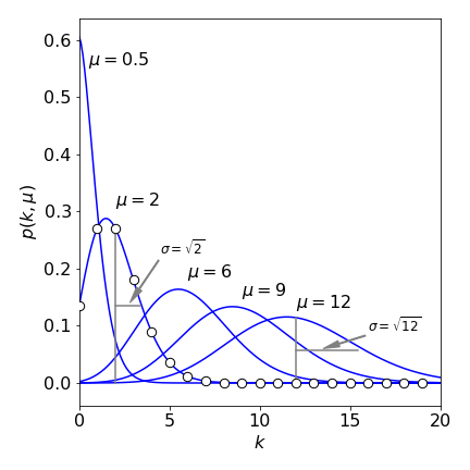
Figure 20e. The Poisson distribution
Notice that, when the mean becomes larger, the distribution resembles a normal distribution and is almost symmetrical. But at small \(\mu\), the distribution is very asymmetrical with the mean always to larger \(k\) than the peak (the mode or most probable value) of the distribution. The standard deviation of the distribution is also shown and this is
where \(\mu\) is the average number of events detected; for instance, the number of photons detected in a given time period at a given wavelength.
The chance of no success, that is of not observing an ‘event’, is \(e^{-\mu}\). The chance of observing exactly one event \(k = 1\) is \(\mu e^{-\mu}\), of exactly two events \(\mu^2 e^{-\mu}/2!\), and of exactly \(k\) events is \(P(k, \mu)\). The chance of observing more than one event is \(1 - e^{-\mu}\) . The sum to infinity is unity, and therefore the distribution is normalized.
(i) Franck-Condon Factors#
One interesting example of this distribution is found in the shape of the envelope of the absorption and emission spectrum of a diatomic molecule that has a harmonic potential in both the ground and electronic excited state. The chance of absorption is found by analysing the Franck-Condon Factor
where \(\psi\) are the Harmonic Oscillator wavefunctions, in the initial \(i\) and final \(f\) energy levels and \(a\) is the displacement of one excited state from the other, i.e. change in bond length between the two electronic states. These wavefunctions are given in section 8.1, equation 18a. Usually only the lowest vibrational level in the ground state is significantly populated because vibrational quanta are usually large (hundreds to a few thousand wavenumbers) compared to thermal energy \(210\;\mathrm{cm^{-1}}\) at room temperature. In this case evaluating the Franck-Condon Factor integral is simplified and the result is a Poisson distribution. The calculation is performed in answering question 4.64 in the integration chapter. The Franck-Condon Factor is
where \(S = \mu\omega a^2/2\hbar\) is called the Huang-Rhys factor and \(\mu\) is the reduced mass of the atoms in the vibration of frequency \(\omega\).
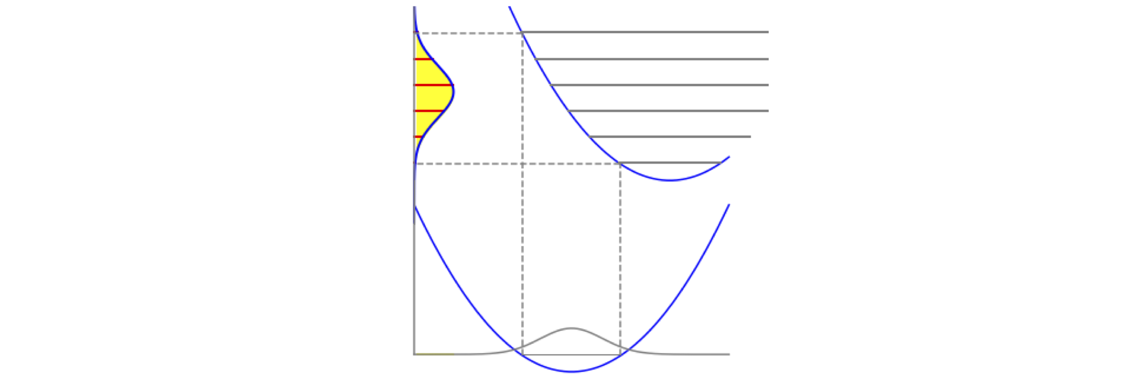
Figure 20f. Harmonic, displaced Potential energy profiles. The spectrum is sketched on the left with the envelope in yellow.
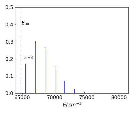
Figure 20d. Calculated spectrum for CO.The size of the absorption lines follows the Poisson distribution.
(ii) Sequential rate equations#
A concatamer of identical proteins can be unfolded one at a time using an atomic force microscope (AFM). Each protein unfolds with the same rate constant. The scheme is \(p_1 \to p_2\to p_3 \to \cdots\). As the rate constant for any step is the same the chance that the transition from protein, \(n\to m\) is Poisson distributed. The calculation is described in full in chapter 10 (Differential equations) section 7. As the rate constants are all the same the unfolding is not sequential so any protein has the same chance of unfolding at a given applied force from the AFM.
(iii) Poisson distribution derived from the binomial#
The binomial distribution can be simplified to produce the Poisson distribution when \(n\to \infty, p \to 0\) but \(\mu\) is constant. The binomial distribution is
which is the total probability of choosing \(m\) objects from \(n\) positions and \(p\) is the (fixed) chance of choosing any one. If we imagine putting particles into boxes as described for 96 well plates in section 9.19, the probability is \(p=1/N\) for \(N\) wells and the average is \(\mu=np\) which means \(n=\mu N\). Substituting for \(p\) gives
We now rearrange this equation and simplify using elementary steps (Haken 1978). The most difficult step is to notice that
using this in the Binomial distribution gives
Now we rearrange this equation and split the last term into powers of \(n\) and \(-k\)
now dividing by \(n^k\) in the fraction gives
The first term remains as it is and the term underlined as A becomes the definition of an exponential when \(n\to \infty\), i.e.
and the term B becomes \(1\) as \(n\to \infty\). This completes the conversion to the Poisson distribution
giving
9.26 Multinomial distribution#
The binomial distribution is concerned with selecting between two classes: success and failure; but the choices need not be restricted to two classes. We have already calculated the chance of observing groups of objects or events, such as the chance of 3 GLY, 3 ILE, etc. in the protein sequence in Section 9.3. When there are several choices the multinomial distribution is required and is
where \(p_i\) is the probability of choosing any object from the \(n\) boxes and \(m_i\) are the numbers in each of \(r\) groups.
In the calculation of the Maxwell - Boltzmann distribution, \(n\) objects are placed into \(s\) identical boxes. The distribution becomes
from which the \(m_i\) has to be found and the distribution is maximized subject to the restriction that both the number of particles and the total energy are constant. This is usually done by taking the log of the distribution and, as each \(m_i\) is large using Stirling’s approximation for \(m_i!\). The constraints are dealt with using the method of Lagrange multipliers see chapter 3.11. The full calculation can be found in textbooks on statistical mechanics.
9.27 Genetics#
Mendel discovered that pure bred but different strains of peas gave rise to offspring that showed different features but did so in definite proportions. His peas had yellow and green seeds, but 75.05% of the offspring in 8023 trials were yellow, and the remainder, green. Others have since found very similar numbers in even larger trials and in other organisms, such as fruit flies or mice (Maynard Smith 1995). The genetic information we now know is encoded in DNA. The regions involved in transmitting genetic information are called genes, and these form part of a chromosome of which several different types are present in an organism.
We are familiar with the observation that the probability with which molecules react is exponentially distributed, which is expressed in a first-order rate equation, the rate being probability/time. In genetics, the situation is entirely different. The probability distribution is flat and the chance that genes mix genetic information occurs with the same constant probability as if they were selected out of boxes, each one being equally probable. Although these genes ‘mix’ during reproduction, they still retain their own identity and are passed down through the generations. An individual needs two genes to express a trait; yellow vs green seeds or stumpy vs normal wings in a fruit fly, and these mix freely from both parents to produce offspring. These traits are usually called phenotypes. The traits the offspring show are expected to be those of the parents, but depending on the genetic make up (genotype) of the parent, some traits appear less than would be expected from simple numerology. The reason for this is that some genes are recessive to others, which are called dominant, and therefore a characteristic trait does not manifest itself in the presence of a dominant gene. Only when the genotype is examined can the true make-up of an individual be found.
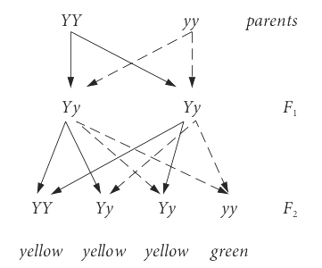
Figure 21. Genetic make-up after two generations (after Maynard Smith 1995). The yellow colour in pea seeds is dominant over green and occurs in the ratio 3:1, although this is not reflected in the genetic make-up.
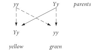
Figure 22 A cross between YY and Yy plants.
If the two genes from each parent are described as Y or y and G or g they can be arranged in a diagram. The uppercase letter indicates a dominant gene, the lower case a recessive. Starting with the pure strains YY and yy, which are called homozygous, the first generation (F1) are heterozygous Yy. If these are now bred, the homozygous reappear with the heterozygous, Figure 21.
Because the yellow colour in the pea seeds is dominant over the green, although this is not reflected in the genetic make-up (the genotype), the chance of observing yellow peas is therefore \(75\)%, which is very close to that observed experimentally. The chance of observing YY and yy genotypes is \(1/4\) in each case, and of the hybrid Yy, \(1/2\), because the genes mix freely but retain their own identity, rather like atoms do in forming a molecule. The yellow seeded plants are present in the ratio 3:1 over the green ones. The phenotype ratio yellow to green is therefore \(3:1\), or put another way, yellow seeded plants are expected to be observed on average in \(3/4\) of all experiments. If a homozygous plant is crossed with a heterozygous one, the chances that green and yellow seeded plants will be produced are equal.
(i) Chance of observing equal numbers#
If, say, \(n= 20\) experiments are performed it should not be assumed that exactly equal numbers of green and yellow seeded plants will be observed since the number of experiments are small and many factors may influence what the plant looks like. This ‘noise’ means that accurate and precise ratios are only produced after averaging a large number of experiments. The numbers could range from \(0 \to 20\) but the average should be \(10\) with the actual probabilities being distributed according to the binomial theorem. The chance (frequency) of observing \(m\) green plants is then from the binomial distribution
which works out to be a very small number, \(<2 \times 10^{-5}\) of observing either \(0\) or \(20\) green pea seeds. The chance of there being exactly \(10\) plants of each type is \(46189/262144 = 0.1762\) or \(17.6\)%. The chance that the actual result differs by \(\pm 1\) from the average value of \(10\) is
which is approximately a \(50\)% chance that the numbers of peas produced will be \(9, 10\), or \(11\) and a \(50\)% chance that they will be greater or smaller than these numbers. If the number of experiments is increased to \(2000\), then there is only a \(5.3\)% chance that the average number will not be between \(1001\) and \(999\).
(ii) The Punnett square#
The Punnett square or matrix is a convenient pictorial way of assessing the outcomes of mixing genes. All of the possible genotypes of one parent are placed on the top row, and those of the other parent in the first column and the genotypes of the offspring fill the matrix. The crossing of the F1 hybrids in Fig. 1.21 is represented as
which gives the same result as in figure 21 but in more compact form.
In many cases there are two genes that encode for a phenotype, and we assume that the genes are located on different chromosomes and are therefore independent. We can predict the fraction of the types of offspring of, for example, mice with brown vs white coats, brown being dominant and short vs long tails, short being dominant. The genotypes are labelled as \(B\) and \(b\) for the colour, and \(T\) and \(t\) for the tails, so that the genotypes are \(BT,\; Bt,\; bT,\; bt\), the lower case being recessive. If these animals are mated, the offspring genotypes are shown in the table, where each entry is arranged with \(B/b\) as the first label and \(T/t\) as the second, and the dominant before the recessive.
An offspring’s phenotypes can be characterised using \(X\) to mean \(B/b\) or \(T/t\) as appropriate. The table shows that
(i) \(9/16\) of genotype \((B\;X\;T\;X\;)\) has phenotype: brown, long tailed
(ii) \(3/16\) as \((b\;b\;T\;X )\equiv\) white, long tail
(iii \(3/16\) as \((B\;X\;t\;t)\equiv\) brown,short-tail (shown as bold in the square)
(iv) \(1/16\) as \((b\;b\;t\;t) \equiv\) white short tail.
The phenotype ratios are \(9:3:3:1\) and this was observed by Mendel in his studies of peas.
(iii) The Hardy-Weinberg Law#
As there are dominant and recessive factors (alleles) after many generations why are there any recessive ones left? The answer to this question was worked out by Hardy, apparently while watching a cricket match, and independently by Weinberg in Germany both around 1908.
In using this law some conditions are assumed, first that mating is entirely random, i.e. that there is no preference between individuals in choosing mates and secondly that the numbers involved are very large so that average behaviour is always obtained. Additionally, it is assumed that natural selection has no effect, i.e. that the genes do not change during the generations over which this law applies. Some texts call this ‘law’ the Hardy-Weinberg Equilibrium, although it is not an equilibrium in the usual chemical meaning of the word, it is more like a steady-state as the fraction of the type of individuals, the phenotypes yy, yY and YY, remains constant over the generations. The genotypes are labelled as dominant Y and recessive y.
In forming the Punnet square we have so far assumed that there is an equal fraction of Y and y alleles, but this cannot be the case generally. Suppose instead we start with fractions \(p\) of Y and \(q\) of y and as \(p\) and \(q\) are probabilities (often called frequencies in genetics) it is true that
As there are only two factors Y and y, the equation
also applies. The Punnet square can now be re-written to include these probabilities as,
The hybrid phenotype (yY and Yy) is present as fraction \(2pq\) and the homogeneous ones as fractions \(p^2\) and \(q^2\).
In the next generation the genes are transmitted from the previous one as the fraction
for the recessive allele y and for the dominant one Y as
These are just the same as the original fractions of y and Y thus after the first generation all subsequent generations have the same fixed proportions and so the recessive allele is always present and the dominant one not entirely dominant.
In experiments there is always ‘noise’ added to the data. This is,naturally, also true in genetics experiments and manifests itself as the numbers of each type of phenotype measured. It is then possible to check whether the Hardy-Weinberg still applies in the presence of noise by performing a \(\chi^2\) test. These tests are described in Chapter 13.
(iv) Example#
Suppose that in a population of \(1000\) individuals \(190\) have characteristics that show the the presence of the recessive allele y and \(810\) show the dominant allele Y. Let the probability (frequency) of the recessive allele y be \(q\). The fraction (frequency or probability) of individuals in the population with yy is therefore \(q^2\),
As Y is dominant the number of individuals with this allele (the phenotype), YY and Yy, is \( p^2+2pq \) so cannot be obtained until \(p\) is known. As \(p+q=1\), the dominant allele is present as the fraction \(p = 1 - 0.436 = 0.564, \quad p^2=0.318\) and the fraction of hybrid individuals is therefore \(2pq= 0.491\). The Punnet square becomes
The number of individuals with YY is \(p^2\times 1000 = 318\), those with Yy is \(2pq\times 1000 = 492\) and those with yy are \(q^2\times 1000 = 190\) which make \(1000\) in total as it should.
In the next generation suppose that there are only \(700\) individuals available for study and of these \(133\) have the recessive trait and \(223\) the dominant. We want to know if the Hardy-Weinberg equilibrium holds. The fraction of recessive individuals is
and therefore \(p = 0.564\) both of which are the same as in the previous generation in accord with the Hardy-Weinberg equilibrium. All subsequent generations will have the same composition as the initial amounts, \(q\) and \(p\), for further generations are now fixed.
(v) Example#
The fractions of phenotypes have been measured as yy \(f_{yy}=0.2\), Yy \(f_{Yy}=0.2\) and YY \(f_{YY}=0.6\). The value of \(p\) is therefore
The amount \(f_{Yy}\) is divided by two as this represents \(2pq\) and only half comes from the dominant Y. As \(p+q=1\), therefore \(q = 0.3\). The Punnet square is
In the next generation the amounts transmitted from the previous generation are for the recessive allele y,
and for the dominant one Y as
and these are the same values for \(q\) and \(p\) for the previous generation, which as these are now the starting values for further generations, these amounts remain constant.