Solutions Q 14 - 26

# added here as used later on
%matplotlib inline
import numpy as np
import matplotlib.pyplot as plt
from sympy import *
init_printing()                      # allows printing of SymPy results in typeset maths format
plt.rcParams.update({'font.size': 14})  # set font size for plots

Q14 answer

The series expansion of \(\tan(x)\) is obtained with repeated differentiation and then evaluating each term at \(x = 0\),

\[\displaystyle \frac{d\tan(x)}{dx}=1+\tan^2(x), \quad \frac{d^2\tan(x)}{dx^2}=2\tan(x)(1+\tan^2(x)~)\]

and so on. The series is then

\[\displaystyle \tan(x) = x+\frac{x^3}{3}+\frac{2}{15}x^5+\frac{17}{315}x^7+ \cdots\]

and when multiplied by that for \(\displaystyle e^x\) produces,

\[\displaystyle \left(x + \frac{x^{3}}{3} + \frac{2 x^{5}}{15} + \cdots\right) \left(1 + x + \frac{x^{2}}{2} + \frac{x^{3}}{6} + \frac{x^{4}}{24} + \frac{x^{5}}{120} + \cdots\right)\]

and multiplying out produces

\[\displaystyle e^x\tan(x)=x + x^{2} + \frac{5}{6}x^{3} + \frac{1}{2}x^{4} + \frac{41}{120}x^{5} + \cdots\]

The calculation is trivial using a computer algebra programme; SymPy is used below;

x = symbols('x')  # using sympy
f01 = tan(x)*exp(x)
s = expand(series( f01, x ))
s

Q15 answer

Rearranging produces \(\displaystyle x\frac{(1+x)}{(x-1)^2}=x\frac{(1+x)}{(x-1)(x-1)}=x\frac{(1+x)}{(1-x)^2}\)

where the last term is obtained by multiplying top and bottom by \((-1)\) twice. Using the series expansion formula for the denominator and then multiplying out gives

\[\begin{split}\displaystyle \begin{align}x\frac{(1+x)}{(1-x)^2} &=x(1+x)[1+2x+3x^2 +4x^3 +\cdots] \\ &= x+2x^2 +3x^3 +4x^4 +\cdots +x^2 +2x^3 +3x^4 +\cdots \end{align} \end{split}\]

which produces the required result after some rearranging. As in the last question sympy can do this calculation directly.

Q16 answer

Rearranging the equation and expanding produces,

\[\displaystyle \frac{E}{mc^2}=\left(1-\frac{v^2}{c^2}\right)^{-1/2} \approx 1+\frac{v}{2c}+\frac{3}{8}\frac{v^2}{c^2}+\cdots\]

and at low speeds when \(v/c \lt 1\) then \((v/c)^2 < v/c\) therefore \(E= mc^2(1+v/2c+\cdots)\) which becomes \(E = mc^2\) when \(v \ll 2c\).

Q17 answer

Using the formula \(\displaystyle x=\frac{-b\pm\sqrt{b^2-4ac}}{2a}\) the square root can be expanded provided \(4ac/b^2 \lt 1\) and re-writing as \(\displaystyle x=\frac{ -b\pm b\sqrt{1-4ac/b^2} }{2a} \)

allows the square-root to be expanded. The result is

\[\displaystyle x\approx \frac{b}{2a}\left[ -1\pm\left(1-\frac{2ac}{b^2}-\frac{a^2c^2}{2b^4} -\cdots \right) \right]\]

Because \(b^2 \gg ac\), the terms in \(b^4\) and higher powers will be small. Taking the positive root gives \(x \approx c/b\), and as \(b\) is larger than \(c\) this root will be small. The negative root gives \(x \approx b/a\) which is large.

Q18 answer

Expanding the exponential as a ratio for small \(x\) gives

\[\displaystyle \frac{x}{e^x -1}=\frac{x}{x+x^2/2!+x^3/3!+\cdots }\]

and dividing by \(x\) gives

\[\displaystyle \frac{1}{e^x -1}=\frac{1}{1+x/2!+x^2/6+\cdots }\]

and when \(x \rightarrow 0\) this produces \(1\) as the limit. Separately differentiating top and bottom of the original function according to l’Hopital’s rule (Chapter 3.8) produces \(\displaystyle e^{-x}\) and in the limit \(x \rightarrow 0\) this is \(1\).

Q19 answer

(a) The expansion is \(\displaystyle \sum_{k=1} e^{ikx} = e^{ix} + e^{2ix} + e^{3ix} + e^{4ix} +\cdots \)

Removing the first term and substituting \(\displaystyle e^{inx} = w^n\) gives \(\displaystyle \sum_{k=1}e^{ikx} =e^{ix}(1+w^2 +w^3 +w^4 +\cdots+)\)

This series looks familiar; to check use the table of series expansions (Chapter 5.6.4) or try with SymPy.

w = symbols('w')
series( 1/(1-w),w )

which then gives \(\displaystyle \sum_{k=1}e^{ikx}=\frac{e^{ix}}{1-e^{ix}}\).

(b) The summation \(\sum_{k=1}^\infty e^{ikx}/k\) is very close to the integral of \(\sum_{k=1}^\infty e^{ikx}\) calculated in (a). Integrating this sum multiplied by \(i\) gives

\[\displaystyle i\int\sum\limits_{k=1} e^{ikx} = \sum\limits_{k=1}\frac{e^{ikx}}{k} + c\]

Integrating the result from part (a) also multiplied by \(i\) gives

\[\displaystyle i\int\frac{e^{ix}}{1-e^{ix}}dx = i\int\frac{1}{-1+e^{-ix} }dx=-\ln(1-e^{ix})\]

Q20 answer

The expansion is

\[\begin{split}\displaystyle \begin{align}\sum\limits_{k=1}^\infty (1-p)p^{k-1} &=(1-p)\sum\limits_{k=1}^\infty p^{k-1}\\ &=(1-p)(1+p+p^2 +p^3 +\cdots) =1+p+p^2 \cdots -p-p^2 -\cdots = 1\end{align}\end{split}\]

where the result is obtained by canceling terms. Instead of canceling the series expansion \(1/(1-p)=1+p+p^2 +\cdots\) could be used directly.

The average is calculated as \(\langle k \rangle = (1 - p)\sum\limits_{k=1}^\infty kp^{k-1}\) and a denominator is not needed because the distribution is normalized.

\[\begin{split}\displaystyle \begin{align} \langle k \rangle &= (1 - p)\sum\limits_{k=1}^\infty kp^{k-1} = (1-p)(1+2p+3p^2 +4p^3 +\cdots+) \\& =1+2p+3p^2 +4p^3 +\cdots -p-2p^2 -3p^3 -4p^4 \\& = 1 + p + p^2 + p^3 + \cdots = 1/(1 - p) \end{align}\end{split}\]

and this last result could also have been obtained directly by differentiating both sides of \(\sum_{k=1}^\infty p^k =1/(p-1)\) with respect to \( p\).

The average \(\langle k^2 \rangle\) is

\[\begin{split}\displaystyle \begin{align} \langle k^2 \rangle =(1-p)\sum_{k=1}^\infty k^2p^{k-1}& =(1-p)(1+4p+9p^2 +16p^3 +\cdots +) \\& =1+4p+9p^2 +16p^3 +\cdots -p-4p^2 -9p^3 -16p^4 \\& =1+3p+5p^2 +7p^3 +\cdots \end{align} \end{split}\]

The final series is the sum \(\displaystyle 1+\sum_{k=1}(2k+1)p^k\) as may be seen by putting \(k = 1, 2,\cdots\). To sum this use the results for \(\displaystyle \sum_{k=1} kp^k\) and \(\displaystyle \sum_{k=1} p^k\) both of which have been met before or are in the table. Alternatively SymPy could be used.

k, p = symbols('k, p')
s =  (1 - p)*summation(k**2*p**(k - 1),(k,1,oo)) 
simplify(s)

\[\begin{split}\displaystyle \begin{cases} \frac{p + 1}{\left(p - 1\right)^{2}} & \text{for}\: p > -1 \wedge p < 1 \\\left(-1 + \frac{1}{p}\right) \sum_{k=1}^{\infty} k^{2} p^{k} & \text{otherwise} \end{cases}\end{split}\]

The standard deviation is \(\displaystyle \sqrt{\langle k^2 \rangle - \langle k \rangle^2} = \frac{\sqrt{p}}{p-1}\) which for large \(p\) becomes smaller but only as as \(1/\sqrt p\) as \(p\) increases. This behaviour is similar to that of repeated measurements reducing standard deviation as \(1/\sqrt N\).

Q21 answer

The function is rewritten as \((\sin(x)/x)^2\) and expanding the \(\sin(x)\) as a Taylor series about \(x = 0\) and dividing by \(x\) produces,

\[\displaystyle \frac{\sin(x)}{x}=1-\frac{x^2}{3!}+\frac{x^4}{5!}+ \cdots \]

squaring the first three terms

\[\displaystyle \frac{\sin^2(x)}{x^2}=1-\frac{x^2}{3}+\frac{2x^4}{45}-\cdots \]

which produces \((\sin(x)/x)^2 \to 1\) when \(x \to 0\) because all the squared and higher terms are small compared to unity. The graph is shown below. The maximum is \(1\), as predicted, and there are repeated zeros at \(\pm n\pi\) where \(n\) is an integer because \(\sin(\pm n\pi) = 0\). These are also shown on the next plot.

# calculation of sinc function
fig1 = plt.figure(figsize=(5,4))
plt.rcParams.update({'font.size': 16})  # set font size for plots

x = np.linspace(-3*np.pi,3*np.pi,100)
sinc2 = lambda x: (np.sin(x)/x)**2
plt.plot(x,sinc2(x),color='blue')
for i in range(1,4):
    v = i*np.pi
    plt.axvline( v,linestyle='--',color='gray',linewidth=1)
    plt.axvline(-v,linestyle='--',color='gray',linewidth=1)
plt.xlabel(r'$x$')
plt.ylabel(r'$\sinc^2(x)$')
plt.axhline(0,color='gray',linewidth=1)
plt.show()

---------------------------------------------------------------------------
ParseFatalException                       Traceback (most recent call last)
File ~/Library/Python/3.9/lib/python/site-packages/matplotlib/_mathtext.py:1983, in Parser.parse(self, s, fonts_object, fontsize, dpi)
   1982 try:
-> 1983     result = self._expression.parseString(s)
   1984 except ParseBaseException as err:

File ~/Library/Python/3.9/lib/python/site-packages/pyparsing/core.py:1141, in ParserElement.parse_string(self, instring, parse_all, parseAll)
   1139     else:
   1140         # catch and re-raise exception from here, clearing out pyparsing internal stack trace
-> 1141         raise exc.with_traceback(None)
   1142 else:

ParseFatalException: Unknown symbol: \sinc, found '\'  (at char 0), (line:1, col:1)

The above exception was the direct cause of the following exception:

ValueError                                Traceback (most recent call last)
File ~/Library/Python/3.9/lib/python/site-packages/IPython/core/formatters.py:339, in BaseFormatter.__call__(self, obj)
    337     pass
    338 else:
--> 339     return printer(obj)
    340 # Finally look for special method names
    341 method = get_real_method(obj, self.print_method)

File ~/Library/Python/3.9/lib/python/site-packages/IPython/core/pylabtools.py:151, in print_figure(fig, fmt, bbox_inches, base64, **kwargs)
    148     from matplotlib.backend_bases import FigureCanvasBase
    149     FigureCanvasBase(fig)
--> 151 fig.canvas.print_figure(bytes_io, **kw)
    152 data = bytes_io.getvalue()
    153 if fmt == 'svg':

File ~/Library/Python/3.9/lib/python/site-packages/matplotlib/backend_bases.py:2314, in FigureCanvasBase.print_figure(self, filename, dpi, facecolor, edgecolor, orientation, format, bbox_inches, pad_inches, bbox_extra_artists, backend, **kwargs)
   2308     renderer = _get_renderer(
   2309         self.figure,
   2310         functools.partial(
   2311             print_method, orientation=orientation)
   2312     )
   2313     with getattr(renderer, "_draw_disabled", nullcontext)():
-> 2314         self.figure.draw(renderer)
   2316 if bbox_inches:
   2317     if bbox_inches == "tight":

File ~/Library/Python/3.9/lib/python/site-packages/matplotlib/artist.py:74, in _finalize_rasterization.<locals>.draw_wrapper(artist, renderer, *args, **kwargs)
     72 @wraps(draw)
     73 def draw_wrapper(artist, renderer, *args, **kwargs):
---> 74     result = draw(artist, renderer, *args, **kwargs)
     75     if renderer._rasterizing:
     76         renderer.stop_rasterizing()

File ~/Library/Python/3.9/lib/python/site-packages/matplotlib/artist.py:51, in allow_rasterization.<locals>.draw_wrapper(artist, renderer)
     48     if artist.get_agg_filter() is not None:
     49         renderer.start_filter()
---> 51     return draw(artist, renderer)
     52 finally:
     53     if artist.get_agg_filter() is not None:

File ~/Library/Python/3.9/lib/python/site-packages/matplotlib/figure.py:3069, in Figure.draw(self, renderer)
   3066         # ValueError can occur when resizing a window.
   3068 self.patch.draw(renderer)
-> 3069 mimage._draw_list_compositing_images(
   3070     renderer, self, artists, self.suppressComposite)
   3072 for sfig in self.subfigs:
   3073     sfig.draw(renderer)

File ~/Library/Python/3.9/lib/python/site-packages/matplotlib/image.py:131, in _draw_list_compositing_images(renderer, parent, artists, suppress_composite)
    129 if not_composite or not has_images:
    130     for a in artists:
--> 131         a.draw(renderer)
    132 else:
    133     # Composite any adjacent images together
    134     image_group = []

File ~/Library/Python/3.9/lib/python/site-packages/matplotlib/artist.py:51, in allow_rasterization.<locals>.draw_wrapper(artist, renderer)
     48     if artist.get_agg_filter() is not None:
     49         renderer.start_filter()
---> 51     return draw(artist, renderer)
     52 finally:
     53     if artist.get_agg_filter() is not None:

File ~/Library/Python/3.9/lib/python/site-packages/matplotlib/axes/_base.py:3106, in _AxesBase.draw(self, renderer)
   3103         a.draw(renderer)
   3104     renderer.stop_rasterizing()
-> 3106 mimage._draw_list_compositing_images(
   3107     renderer, self, artists, self.figure.suppressComposite)
   3109 renderer.close_group('axes')
   3110 self.stale = False

File ~/Library/Python/3.9/lib/python/site-packages/matplotlib/image.py:131, in _draw_list_compositing_images(renderer, parent, artists, suppress_composite)
    129 if not_composite or not has_images:
    130     for a in artists:
--> 131         a.draw(renderer)
    132 else:
    133     # Composite any adjacent images together
    134     image_group = []

File ~/Library/Python/3.9/lib/python/site-packages/matplotlib/artist.py:51, in allow_rasterization.<locals>.draw_wrapper(artist, renderer)
     48     if artist.get_agg_filter() is not None:
     49         renderer.start_filter()
---> 51     return draw(artist, renderer)
     52 finally:
     53     if artist.get_agg_filter() is not None:

File ~/Library/Python/3.9/lib/python/site-packages/matplotlib/axis.py:1316, in Axis.draw(self, renderer, *args, **kwargs)
   1310 # Scale up the axis label box to also find the neighbors, not just the
   1311 # tick labels that actually overlap.  We need a *copy* of the axis
   1312 # label box because we don't want to scale the actual bbox.
   1314 self._update_label_position(renderer)
-> 1316 self.label.draw(renderer)
   1318 self._update_offset_text_position(tlb1, tlb2)
   1319 self.offsetText.set_text(self.major.formatter.get_offset())

File ~/Library/Python/3.9/lib/python/site-packages/matplotlib/artist.py:51, in allow_rasterization.<locals>.draw_wrapper(artist, renderer)
     48     if artist.get_agg_filter() is not None:
     49         renderer.start_filter()
---> 51     return draw(artist, renderer)
     52 finally:
     53     if artist.get_agg_filter() is not None:

File ~/Library/Python/3.9/lib/python/site-packages/matplotlib/text.py:688, in Text.draw(self, renderer)
    685 renderer.open_group('text', self.get_gid())
    687 with self._cm_set(text=self._get_wrapped_text()):
--> 688     bbox, info, descent = self._get_layout(renderer)
    689     trans = self.get_transform()
    691     # don't use self.get_position here, which refers to text
    692     # position in Text:

File ~/Library/Python/3.9/lib/python/site-packages/matplotlib/text.py:322, in Text._get_layout(self, renderer)
    320 clean_line, ismath = self._preprocess_math(line)
    321 if clean_line:
--> 322     w, h, d = _get_text_metrics_with_cache(
    323         renderer, clean_line, self._fontproperties,
    324         ismath=ismath, dpi=self.figure.dpi)
    325 else:
    326     w = h = d = 0

File ~/Library/Python/3.9/lib/python/site-packages/matplotlib/text.py:97, in _get_text_metrics_with_cache(renderer, text, fontprop, ismath, dpi)
     94 """Call ``renderer.get_text_width_height_descent``, caching the results."""
     95 # Cached based on a copy of fontprop so that later in-place mutations of
     96 # the passed-in argument do not mess up the cache.
---> 97 return _get_text_metrics_with_cache_impl(
     98     weakref.ref(renderer), text, fontprop.copy(), ismath, dpi)

File ~/Library/Python/3.9/lib/python/site-packages/matplotlib/text.py:105, in _get_text_metrics_with_cache_impl(renderer_ref, text, fontprop, ismath, dpi)
    101 @functools.lru_cache(4096)
    102 def _get_text_metrics_with_cache_impl(
    103         renderer_ref, text, fontprop, ismath, dpi):
    104     # dpi is unused, but participates in cache invalidation (via the renderer).
--> 105     return renderer_ref().get_text_width_height_descent(text, fontprop, ismath)

File ~/Library/Python/3.9/lib/python/site-packages/matplotlib/backends/backend_agg.py:238, in RendererAgg.get_text_width_height_descent(self, s, prop, ismath)
    234     return w, h, d
    236 if ismath:
    237     ox, oy, width, height, descent, font_image = \
--> 238         self.mathtext_parser.parse(s, self.dpi, prop)
    239     return width, height, descent
    241 font = self._prepare_font(prop)

File ~/Library/Python/3.9/lib/python/site-packages/matplotlib/mathtext.py:226, in MathTextParser.parse(self, s, dpi, prop)
    222 # lru_cache can't decorate parse() directly because prop
    223 # is mutable; key the cache using an internal copy (see
    224 # text._get_text_metrics_with_cache for a similar case).
    225 prop = prop.copy() if prop is not None else None
--> 226 return self._parse_cached(s, dpi, prop)

File ~/Library/Python/3.9/lib/python/site-packages/matplotlib/mathtext.py:247, in MathTextParser._parse_cached(self, s, dpi, prop)
    244 if self._parser is None:  # Cache the parser globally.
    245     self.__class__._parser = _mathtext.Parser()
--> 247 box = self._parser.parse(s, fontset, fontsize, dpi)
    248 output = _mathtext.ship(box)
    249 if self._output_type == "vector":

File ~/Library/Python/3.9/lib/python/site-packages/matplotlib/_mathtext.py:1985, in Parser.parse(self, s, fonts_object, fontsize, dpi)
   1983     result = self._expression.parseString(s)
   1984 except ParseBaseException as err:
-> 1985     raise ValueError("\n".join(["",
   1986                                 err.line,
   1987                                 " " * (err.column - 1) + "^",
   1988                                 str(err)])) from err
   1989 self._state_stack = None
   1990 self._in_subscript_or_superscript = False

ValueError: 
\sinc^2(x)
^
Unknown symbol: \sinc, found '\'  (at char 0), (line:1, col:1)

<Figure size 500x400 with 1 Axes>

Figure 24. Graph of \((\sin(x)/x)^2\). The vertical lines are at the zeros of the function that occur at \(n\pm \pi\) where \(n\) = 1, 2, \(\cdots\).

---

Q22 answer

(a) The power series expansion has the form \(\displaystyle f(s)=e^{-s^2}=1-sf^{'}(0)+\frac{s^2}{s!}f^{''}(0)+\cdots \) and the derivatives are

\[\begin{split}\displaystyle \begin{align}f'(s) &= -2sf(s),\quad f''(s) = -2f(s) - 2sf'(s) \\ f'''(s) &= -2f'(s) - 2f'(s) - 2sf''(s),\quad f^4(s) = -4f''(s) - 2f'''(s) - 2sf'''(s) \end{align}\end{split}\]

When \(s = 0\) the Maclaurin series is \(\quad f(0) = 1,\quad f'(0) = 0,\quad f''(0) = -2,\quad f'''(0) = 0,\quad f^4(0) = 12\) where each odd-power derivative is zero. Substituting into the series expansion for \(\displaystyle e^{\large{{-s^2}}}\) gives

\[\displaystyle e^{\large{{-s^2}}} \approx 1-\frac{s^2}{1!} +\frac{s^4}{2!} -\frac{s^6}{3!} +\frac{s^8}{4!} \cdots\]

and integrating this series term by term produces,

\[\displaystyle \text{erf}(x) \approx \frac{2}{\sqrt{\pi}}\int\limits_0^x 1-s^2 + \frac{s^4}{2} -\cdots ds = \frac{2}{\sqrt{\pi}}\left[ x- \frac{x^3}{3} +\frac{x^5}{10}-\frac{x^7}{42} +\frac{x^9}{216}-\cdots \right] \]

(b) The next calculation compares approximation with exact values

from scipy.special import erf   # import error function as this is not 
                                # otherwise defined in python

apprx_erf = lambda x: (2/np.sqrt(np.pi))*(x - x**3/3 + x**5/10 - x**7/42 + x**9/216)

print('{:s}'.format('   x       erf(x)   approx erf(x)'))
for x in [0.1,0.5,0.8,1.0]:
    print('{:6.3f}{:12.8f}{:12.8f}'.format( x,erf(x),apprx_erf(x)))

   x       erf(x)   approx erf(x)
 0.100  0.11246292  0.11246292
 0.500  0.52049988  0.52050028
 0.800  0.74210096  0.74216826
 1.000  0.84270079  0.84344850

which shows that the series approximation is quite good even up to \(x = 1\) if not too much precision is required. Naturally increasing the number of terms in the series will improve the precision.

Q23 answer

The series expansion can be worked out from first principles or looked up and based on \(\displaystyle \frac{1}{1-ax} =1+ax+(ax)^2 +(ax)^3 +\cdots\) with \(a=1,\,x=t^2\) and provided that \(t^2 \lt 1\) the expansion will be valid;

\[\displaystyle \frac{1}{1-t^2} \approx 1+t^2 +t^4 +t^6 +\cdots\]

Integrating term by term gives \(\displaystyle \tanh^{-1}(x) \approx \left[t + t^3/3 + t^5/5 + \cdots \right]_0^{x} = x + x^3/3 + x^5/5 + \cdots\).

This series can be summed and compared to an accurate calculation;

x = 0.5
atanh = sum( [x**n/n for n in range(1,15,2)] )    # make list then sum, increment by 2 from 1 to 15
print('{:s}{:f}{:s}{:f}'.format('tanh(',x,') summation ',atanh))
print('{:s}{:f}{:s}{:f}'.format('tanh(',x,') direct    ',np.arctanh(x)))   

tanh(0.500000) summation 0.549304
tanh(0.500000) direct    0.549306

Q24 answer

Expanding \(\psi\) about some arbitrary point \(x_0\) and then adding and subtracting \(h\) from \(x\) gives

\[\displaystyle \psi(x)=\psi(x_0)+(x-x_0)\left( \frac{d\psi}{dx} \right)_{x_0} +\frac{(x-x_0)^2}{2!}\left( \frac{d^2\psi}{dx^2} \right)_{x_0} + \cdots\]

\[\displaystyle \psi(x+h)=\psi(x_0)+(x+h-x_0)\left( \frac{d\psi}{dx} \right)_{x_0} +\frac{(x+h-x_0)^2}{2!}\left( \frac{d^2\psi}{dx^2} \right)_{x_0} + \cdots\]

\[\displaystyle \psi(x-h)=\psi(x_0)+(x-h-x_0)\left( \frac{d\psi}{dx} \right)_{x_0} +\frac{(x-h-x_0)^2}{2!}\left( \frac{d^2\psi}{dx^2} \right)_{x_0} + \cdots\]

Combining the terms as in the question, removes \(x_0\) and greatly simplifies the expression, and produces the required result;

\[\begin{split}\displaystyle \begin{align}\psi(x + h) + \psi(x - h) - 2\psi(x)&=\frac{D^2\psi(x)}{2}[(x+h-x_0)^2 +(x-h-x_0)^2-2(x-x_0)^2]\\&=h^2D^2\psi(x)\end{align}\end{split}\]

Q25 answer

The expansion is closely related to a standard one; see table of series expansions, giving \(\displaystyle (1+u^2)^{-1} =1-u^2 +u^4 -u^6 +\cdots\)

Integrating produces

\[\displaystyle \int_0^x\frac{dx}{1+u^2} \approx x - \frac{x^3}{3}+\frac{x^5}{5}-\frac{x^7}{7}+\cdots (-1)^{n+1}\frac{x^{2n-1}}{2n-1}+\cdots\]

Trying values of x gives \(\displaystyle \tan^{-1}(1) = \pi/4\), which is the same as saying that the tangent of \(45^\text{o}\) is 1, which of course you already knew. The series is therefore

\[\displaystyle \frac{\pi}{4}=\sum\limits_{n=1}^\infty\frac{(-1)^{n+1}}{2n-1}\]

Evaluating this you will find that it converges very, very slowly; the alternating positive and negative terms are clearly the cause of this therefore this is a very poor way to find \(\pi\), even to a few decimal places, as shown below where even 500 terms produce a poor estimation.

i = 500  # number of terms in summation
s = 4*sum( [ (-1)**(n+1.0)/(2*n-1.0) for n in range(1,i)]  )
print('{:s}{:20.16f}'.format('series  ', s))
print('{:s}{:20.16f}'.format('accurate', np.pi))

series    3.1435966595937890
accurate  3.1415926535897931

Q26 answer

Expanding the cosine inside the integral gives

\[\displaystyle \int_0^x \cos(x^3)dx = x - \frac{x^7}{7\cdot2!}+\frac{x^{13}}{13\cdot4!} -\frac{x^{19}}{19\cdot6!}+\cdots=\sum\limits_{n=0}^\infty\frac{(-1)^nx^{6n+1}}{(6n+1)(2n!)}\]

where the last summation term is obtained after some guessing and by copying the similar terms for the cosine and cubing and adding 1 to the power, (because we integrated) and also dividing by 6\(n\) + 1 for the same reason.

In calculating this series, several terms will be needed and using sympy makes it relatively easy. A variable \(s\) holds the sum and it is added to each time round the loop. The result is plotted so that it can be seen how quickly or not the series converges to a result.

# Use our own factorial function using recursion; good for small values of n 
#-------------------
def fact(n):
    if n == 0 or n == 1:
        return 1
    else:
        return n*fact(n-1)
#--------------------

nmax = 20
x    = 2.0
val  = [0.0 for i in range(nmax)]
s    = 0.0
for n in range(nmax):
    s = s + (-1)**n*x**(6*n + 1)/( (6*n + 1)*(fact(2*n)) )
    val[n] = s
    plt.scatter(n, val[n], s=50,color='blue',facecolor='white',zorder=10)
    #print('{:4d}{:16.10f}'.format(n,s))   # print each value if needed
    pass
print('{:s} {:f} {:s} {:f}'.format('sum to ',x, ' is ',s ))
plt.plot(val,color='blue',linewidth=1)
plt.xlabel('n')
plt.ylabel('summed value')
plt.axhline(0,color='grey',linewidth=1)
plt.show()

sum to  2.000000  is  0.855475

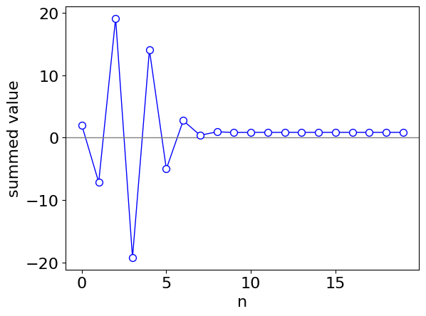
Figure 25a. Terms in the summation as it extends with powers of \(n\).

---

By direct integration the similar answer is obtained.

x = symbols('x')
ans = integrate(cos(x**3), (x,0,2),conds='none')
ans.evalf()

If a simple summation expression cannot be found, you can always try making a series with SymPy. Then repeat the calculation with more terms in the series.

Generally, one would proceed cautiously with this method. Some functions, such as the one examined here, are ‘perverse’ and may take hundreds of terms to converge and then the risk of numerical ‘rounding’ errors is large, which occurs when two large and similar real numbers are subtracted. In this example, the function oscillates wildly with increasing frequency as \(x\) becomes larger; this means that numerical errors dominate the integration when the upper limit approaches \(3\). Preferably a proper numerical method, see Chapters 10 & 11 or the Euler-Maclaurin formula, Section 7, should be used.

# calculate series of a general function  in z and plot with original function. 
# Try some functions such as cos(z^3)sin(z). 
# this is a ***slow***  calculation as the symbolic result is found first.

z   = symbols('z')                          # define symbolic variable                         
f01 = cos(z**3)*exp(-z)                     # function to expand into series

num_terms = 150
s   =  series(f01,z,0,num_terms).removeO()  # get series and remove 'big O' as last term 150 terms in series
f03 = lambdify(z,s,'numpy')                 # make into numpy function after series expansion

numx = 1000
maxx = 4
x = np.linspace(0,maxx,numx)                # make set of numx points starting at 0 ending at 4
y = [ f03(x[i]) for i in range(numx) ]      # calculate function at points x[i] and put into array for plotting

plt.plot(x,y,color='red',label='series')
afun = lambdify(z,f01,'numpy')              # make original function into numpy function
plt.plot(x,afun(x),color='blue',label = f01)
plt.axis([0,maxx,-0.5,1.25])
plt.legend()
plt.title('series expansion & its function ')
plt.show()

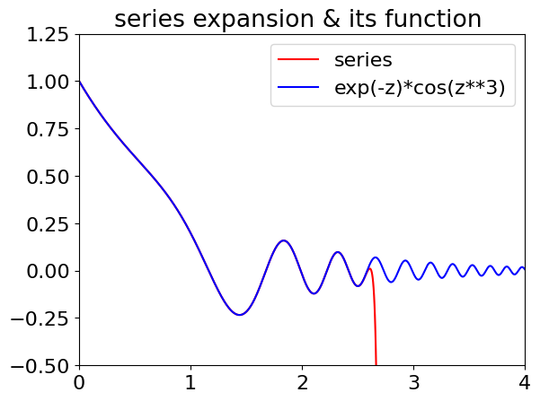
Figure 25b. \(\cos(x^3)e^{-x}\) and its series expansion up to \(x^{150}\). Notice how the series solution (red line) suddenly fails at about \(x = 2.7\). This will cause huge errors in the integration if the limit is taken this far.