
Solutions Q1 - 6
Contents
Solutions Q1 - 6#
%matplotlib inline
import numpy as np
import matplotlib.pyplot as plt
from sympy import *
init_printing()                      # allows printing of SymPy results in typeset maths format
plt.rcParams.update({'font.size': 16})  # set font size for plots
Q1 answer#
Plotting this curve shows that it oscillates about the x-axis and therefore very many evaluations will be necessary as terms of opposite sign cancel out. Using the mean value method and \(15000\) points, produced a value of \(0.277 \pm 0.005\), which is fairly close to the more accurate estimate of \(0.2705\).
Q2 answer#
Three random numbers are needed for each of \(x,\;y\), and \(z\). A guess of 5000 calculations is made, this may have to be increased if a large error is produced. An accurate integration gives 11.04148. With 20000 points in the monte-carlo integration a typical value is \(11.044 \pm 0.004\).
# Algorithm: Mean value monte carlo method for a triple integral.

f = lambda x,y,z:np.sqrt(16.0-x**2-y**2-z**2)
n = 20000                                      # guess number of calculations
lim1 = 0.0
lim2 = 2.0
lim3 = 0.0
lim4 = 1.0
lim5 = 0.0
lim6 = 1.5
s = 0.0
s2= 0.0
for i in range(n):
    x = (lim2 - lim1)*np.random.ranf() + lim1
    y = (lim4 - lim3)*np.random.ranf() + lim3
    z = (lim6 - lim5)*np.random.ranf() + lim5
    s = s + f(x,y,z)
    s2= s2+ f(x,y,z)**2
    pass

int_f =   (lim4 - lim3)*(lim2 - lim1)*(lim6 - lim5)*s/n
int_f2= ( (lim4 - lim3)*(lim2 - lim1)*(lim6 - lim5))**2*s2/n
sig   = np.sqrt( (int_f2 - int_f**2)/n )                     # sqrt( (<x^2>-<x>^2 )/n )
print('{:8.4f} {:s} {:8.4f}'.format( int_f, '+/-',  sig ) )
11.0367 +/- 0.0041
Q3 answer#
If the function chosen is \(\sin(x^2)\) then its integral cannot be inverted easily and is of no use. Therefore, the simple exponential \(e^{-x}\) is chosen. Use the method and algorithm as described in the text, with limits of \(a=0,\; b = 10\), making the ratio \(r = (1 - e^{-t})/(1-e^{-b})\) . The ratio \(f(x)/p(x) =\sin(t^2)\) because the exponential cancels out. The answer, with \(20000\) samples, is \(0.268 \pm 0.003\) which has a smaller variance than the \(0.278 \pm 0.006\) estimated by the mean value method with the same number of samples. The accurate value is \(271\) to \(3\) decimal places.
Q4 answer#
All the preliminary work is now done and making changes to the code in the text gives the result \(0.883 \pm 0.003\); a very similar result to the values obtained by using an exponential distribution illustrated in the text, also with \(5000\) samples. The shape of the function, as long as it generally has the same shape as the function, gives an improved variance compared to simple uniform sampling.
Q5 answer#
(a) The mean value method using Algorithm 2 with \(f = 1/x^{1/2}\) and \(20000\) samples, gives typical values \(1.99 \pm 0.02\) which is close to the true value of \(2.0\). Similar good agreement with the analytic result is found when \(\gamma\) is positive.
(b) Using \(f = 1/x^{0.8}\) gives rather erratic answers, with an average \(4.7 \pm 0.4\), being typical after \(20000\) samples, which is far from the true value of \(5\). After \(10^5\) samples the result has not settled down to a fixed value, nor has it done so after \(10^6\) samples, with a value \(4.7 \pm 0.1\) being typical, which is quite unexpected and unusual behaviour. See figure 20a. Using python/Sympy the correct value is obtained.
The origin of this behaviour would appear to lie in the fact that the function tends to infinity as \(x \to 0\). With an increasing number of samples, there are many \(x\) values close to zero and the large numbers these produce have a disproportionate effect on the integral relative to those at large \(x\), which contribute almost nothing. Importance sampling should correct this effect.
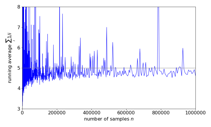
Figure 29. Monte-Carlo calculation of the integral \(\int_0^1 x^\gamma dx\) with \(\gamma =-0.8\) showing that the true average \(5\) is not approached even for a huge number of samples.
(c) The distribution function is \(p(x) = x^\lambda\) where \(\lambda\) has to be chosen to be between zero and \(\gamma\). This function is almost the same as \(f\), and by dividing by \(f\) makes the function integrated much flatter and so has a reduced standard deviation.
The integral is changed to \(\displaystyle \int_0^1 x^\gamma dx=\int_0^1\left(x^{\gamma-\lambda} \right)x^\lambda dx\) and normalising the distribution produces \(\displaystyle \frac{1}{N}\int_0^tx^\lambda dx=x^{t+1}=r\) from which \(t = r^{1/(t+1)}\). The normalization constant is \(N = 1/(1 + \lambda)\). The next step is to choose a value for \(\lambda\) and this is done so that \(\gamma -\lambda\) is close to zero because small powers of \(x\) lead to an accurate integration; choosing \(\gamma -\lambda = 0.1\) is a suitable value although other small values could be used. Making these changes and using \(t=\mathrm{rand}()^{1/(\lambda+1)}\); in the importance sampling algorithm after 20000 samples, a value of \(4.996 \pm 0.020\) is obtained. This is now acceptably close to the true value of \(5\). Furthermore, if the difference between \(\lambda\) and \(\gamma\) is made smaller, for instance \(\gamma -\lambda = 0.01\), then the calculation produces \(4.995 \pm 0.008\) after only \(1000\) samples; quite an improvement. Finally, making the difference zero produces the exact result with zero standard deviation. Why is this?
Q6 answer#
Using the mean value method and the functions in the question the integration produces \(B_2= -0.0244 \pm 0.0006\) after \(30000\) samples. The only way to determine convergence in the integral is to repeat it with a larger \(r\) and with more data points, even though the error appears to be small.
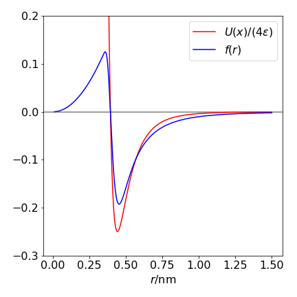
Figure 30. The function to be integrated is \(f(r)\) (blue line) and the potential \(U/4\epsilon\) .