Solutions Q 12-42

# import all python add-ons etc that will be needed later on
%matplotlib inline
import numpy as np
import matplotlib.pyplot as plt
from sympy import *
from scipy.optimize import fsolve
init_printing()               # allows printing of SymPy results in typeset maths format
plt.rcParams.update({'font.size': 14})  # set font size for plots

Q12 answer

Results are mainly calculated as function of function and/or as products.

\(\displaystyle \begin{array}{lll}\\ (a)&\displaystyle \frac{d}{dx}\sin(ax)e^{-bx} = a\cos(ax)e^{-bx}-b\sin(ax)e^{-bx}\\ (b)& \displaystyle\frac{d}{dx}\tanh(x)e^{-bx}=\frac{d}{dx}\frac{\sinh(x)e^{-bx}}{\cosh(x)}=\frac{\cosh(x)e^{-bx}-b\sinh(x)e^{-bx}}{\cosh(x)}-\frac{\sinh^2(x)e^{-bx}}{\cosh^2(x)}\\ (c)&\displaystyle\frac{d}{dx}e^{-2b\sin(x^2)}=-4bx\cos(x^2)e^{-2b\sin(x^2)}\\ (d)& \displaystyle\frac{d}{dx}\ln(a+bx)\cos(ax)=\frac{b}{a+bx}\cos(ax)-a\ln(a+bx)\sin(ax)\\ (e)& \displaystyle\frac{d}{dx}\ln(a+\cos(bx))=-\frac{b\sin(bx)}{a+\cos(bx)}\\ (f)& \displaystyle\frac{d}{dx}\ln(a+b\sin(x))^2=2b\ln(a+b\sin(x))\frac{\cos(x)}{a+b\sin(x)}\\ (g)& \displaystyle\frac{d}{dx}\sqrt{ \cos(e^{x^2}-1) }=-\frac{1}{2\sqrt{\cos(e^{x^2}-1) } }\sin(e^{x^2}-1)2xe^{x^2}\\ \end{array}\)

(h) \(\cosh(y)=x\) is an example of implicit differentiation. The result is \(\displaystyle \sinh(y)\frac{dy}{dx}=1 \) which still contains \(y\) and substituting for \(x\) gives a most unsatisfactory result

\[\displaystyle \sinh(\cosh^{-1}(x))\frac{dy}{dx}=1\]

The initial result can be simplified using \(\cosh^2(y)-\sinh^2(y)=1\) and gives after substitution and rearrangement

\[\displaystyle \frac{dy}{dx}=\frac{1}{\sqrt{x^2-1}}\]

(i) \(\sin^{-1}\) is called the inverse sine or arcsine, a similar notation applies to cosines and tangents. The equation \(y = \sin^{-1}(x/a)\) means \(y\) is the angle such that \(\sin(y) = x/a\). This equation is not the same as \(\displaystyle y=(\sin(x/a))^{-1}=\frac{1}{\sin(x/a)}\) which may be seen from the next part of this question.

Rearranging to \(\sin(y) = x/a\) and (implicitly) differentiating gives \(\displaystyle \cos(y)\frac{dy}{dx}=\frac{1}{a}\). Substituting for \(y\) into this result will produce a very complicated equation. Instead, if \(y\) is thought of as an angle(see Fig.38) it follows that

\[\begin{split}\displaystyle \begin{align}\sin(y) &= x/a &\equiv\qquad \text{ opposite/hypotenuse}\\ \cos(y) &=\sqrt{a^2-x^2}/a &\equiv\qquad \text{ adjacent/hypotenuse}\end{align}\end{split}\]

and consequently

\[\displaystyle \frac{dy}{dx}=\frac{1}{\sqrt{a^2-x^2}}\]

Figure 38. Defining angles

---

(j) \(\displaystyle y=\frac{1}{\sin(x/a)}\) hence \(\displaystyle \frac{dy}{dx}=-\frac{\cos(x/a)}{a\sin^2(x/a)}\)

(k) \(\displaystyle \frac{d}{dq}(\sin^2(q)+q^2\cos(q))=2\sin(q)\cos(q)+2q\cos(q)-q^2\sin(q)\)

Q13 answer

(a) Taking logs gives \(\ln(y)=y\ln(x)\) and differentiating

\[\displaystyle \frac{1}{y}\frac{dy}{dx}=\frac{dy}{dx}\ln(x)+\frac{y}{x} \to \frac{dy}{dx}=\frac{y^2}{x(1-y\ln(x))}\]

(b) again taking logs gives \(\ln(x)=y\ln(y)\) hence \(\displaystyle \frac{1}{x}=\frac{dy}{dx}(\ln(y)+1)\)

(c) \(\ln(y)=x\ln(x)\) therefore \(\displaystyle \frac{1}{y}\frac{dy}{dx}=\ln(x)+1\). At the minimum \(dy/dx=0\) then \(\ln(x)=-1\) or \(x=e^{-1}\) and minimum \(y\) is \(y=(e^{-1})^{e^{-1}}\). If you plot \(x^x\) it looks a bit like a harmonic potential.

Q14 answer

Differentiating once by \(a\) gives \(\displaystyle \frac{d}{da}\int e^{ax}dx=\int\frac{\partial}{\partial a}e^{ax} dx=\int xe^{ax}dx\)

and again \(\displaystyle \frac{d}{da}\int xe^{ax}dx=\int\frac{\partial}{\partial a}xe^{ax} dx=\int x^2e^{ax}dx\)

By induction it follows that

\[\displaystyle \frac{d^n}{da^n}\int e^{ax}dx=\int\frac{\partial^n}{\partial a^n}e^{ax} dx=\int x^ne^{ax}dx\]

Because \(\displaystyle \int e^{ax}dx=\frac{e^{ax}}{a}\) (see table in chapter on integration) then the differential can be rearranged to

\[\displaystyle \int x^ne^{ax}dx=\frac{d^n}{da^n}\left( \frac{e^{ax}}{a} \right)\]

(b) The similar process as in (a) produces

\[\displaystyle \frac{d^n}{da^n}\left( \frac{\sin(ax)}{a}\right)=\int x^n\sin(ax)dx\]

when \(n\) is odd and when even

\[\displaystyle \frac{d^n}{da^n}\left( \frac{\sin(ax)}{a}\right)=\int x^n\cos(ax)dx\]

Q15 answer

(a) Although it is not too difficult to do the differentiation by hand, Python/SymPy is used not only for this but also to plot the equation. It is easier to make \(x\) and \(y\) functions of \(t\) so that \(t\) can be passed as a parameter;

fig = plt.figure(figsize=(12,5))           # plot using matplotlib 
plt.rcParams.update({'font.size': 16})     # set font size for plots
ax0 = fig.add_subplot(1,2,1)
ax1 = fig.add_subplot(1,2,2)
ax0.set_aspect(1)                          # set aspect ratio = 1

t = np.linspace(-np.pi,np.pi,200)          # set range for t
x = lambda t: np.sin(t) - np.sin(2*t)**3   # numpy invoked by using np, see top of page
y = lambda t: np.cos(t) - np.cos(2*t)**3

ax0.plot(x(t),y(t),color='blue')
ax0.axhline(0,linewidth=1,color='grey')
ax0.axvline(0,linewidth=1,color='grey')
ax0.set_xlabel('x')
ax0.set_ylabel('y')

dxdt= lambda t: np.cos(t) - 6*np.sin(2*t)**2*np.cos(2*t)
ax1.plot(t,dxdt(t),color='red')
ax1.set_xlabel('t')
ax1.set_ylabel('x')
ax1.axhline(0,linewidth=1,color='grey')
ax1.grid(True)
ax1.set_title(r'$dx/dt$')
plt.tight_layout()
plt.plot()

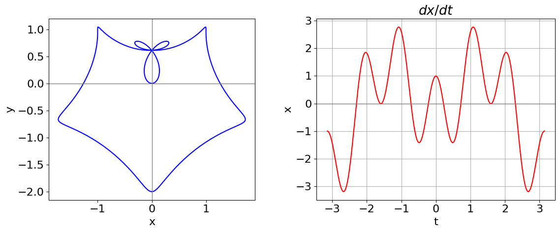
Figure 39. Left: Parametric curve \(x = \sin(t) - \sin^3(2t),\; y = \cos(t) - \cos^3(2t)\). Right: \(\displaystyle \frac{d}{dt} x(t)\) vs \(t\). The zeros in this function are where the vertical tangent is found.

---

# do differentiation symbolically

t, xx, yy = symbols(' t, xx, yy')  # used SymPy 

xx = sin(t) - sin(2*t)**3
yy = cos(t) - cos(2*t)**3

dxdt = diff(xx,t)
dydt = diff(yy,t)
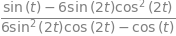
print('dx/dt = ',dxdt)
print('dy/dt = ',dydt)

#calculate dy/dx as the ratio
simplify(dydt/dxdt)

dx/dt =  -6*sin(2*t)**2*cos(2*t) + cos(t)
dy/dt =  -sin(t) + 6*sin(2*t)*cos(2*t)**2

The vertical tangents are found when

\[\displaystyle dx/dt = \cos(t)- 6 \sin^2(2t)\cos(2t) = 0\]

One root (or solution) occurs when \(t = \pm \pi /2\) and then \(x = y = \pm 1\). Other solutions cannot so easily be obtained algebraically: from the figure there are four solutions with \(x \gt 0\) and four with \(x \lt 0\). The remaining calculation has to be done numerically and the Newton - Raphson method, described in Section 10 of this chapter, allows the solutions to be found. These other solutions occur at approximately (\(\pm 0.14096, 0.23310), \,(\pm 0.31522, 0.74867), \,(\pm 1.72690, -0.66474 )\). The code segment below shows how to use the built-in numerical equation solver. Initial guesses close to the solution are needed and convergence need to be checked.

Exercise: Using the Newton - Raphson method find the roots of \(dx/dt\); Use the plot this derivative first to help you find the starting points for the numerical method. Find the horizontal tangents.

# from scipy.optimize import fsolve     # should be included at top of script.

dx = lambda t: np.cos(t) - 6*np.sin(2*t)**2*np.cos(2*t) # function to use

ans = fsolve(dx,0.1,full_output=True)   # 0.1 is initial guess; full_output is used to check convergence.

print(ans[0],ans[-1])
print('coordinates',  x(ans[0]),y(ans[0]) )

[0.2188284] The solution converged.
coordinates [0.14095905] [0.23309729]

Q16 answer

(a) The gradient is, by equation(23), \(\displaystyle \frac{dy}{dx}=-\frac{\cos(t)+\cos(2t)}{\sin(t)+\sin(2t)}\).

(b) The gradient (tangent) is zero when \(\displaystyle \frac{dy}{dt}= 2\cos(t)+2\cos(2t)=0\).

Solving produces several answers which when evaluated are all real within the limits of numerical evaluation and are \(\pm \pi,\; \pm \pi/3\) the latter are \(\pm 1.047\). The larger values are repeated solutions as the function is periodic.

When

\[\displaystyle t = \pi/3,\; y = 2 \sin(\pi /3) + \sin(2\pi /3)=(3\sqrt{3})/2\]

and

\[\displaystyle x = 2 \cos(\pi /3) + \cos(2\pi /3) + 1 = 3/2\]

The equation of the tangent is a straight line \(y = mx + c\), through point \((3/2, (3\sqrt{3}3)/2)\) if the slope is zero \(y = \pm3 \) and these tangents are shown on fig 40.

When \(t = \pi\), the gradient is \(0/0\) and is undefined but tends to \(-\infty\) as \(t \to \pi\).

The horizontal tangent is found when \(dy/dt = 0\) which is given in (b) above. The vertical tangent is

\[\displaystyle dx/dt = -2 \sin(t) - 2 \sin(2t) = 0\]

which has four solutions where \(t = 0,\; \pi,\; \pm 2\pi /3\) which occur at points \((4, 0),\; (0, 0),\; (-1/2, \sqrt{3}/2)\) and \((-1/2, -\sqrt{3}/2)\) respectively.

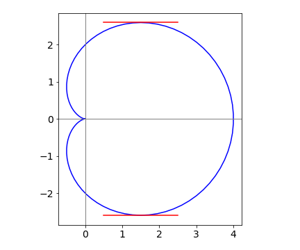
Figure 40. Cardiod with horizontal tangents.

---

# the calculations are shown below
t = symbols(' t', positive = True)      # use SymPy
dydx = cos(t) + cos(2*t)
ans = solve(dydx, t, check = False)     # use check = False so as not to miss root
ans

for j,i in enumerate(ans):
    print((ans[j].evalf()))   # imag part is so small that numbers are real.

zoo
-5.23598775598299
-3.14159265358979
-1.04719755119660
1.04719755119660
3.14159265358979
5.23598775598299

Q17 answer

The differentiation variable is the same as for integration because the integrand has only one variable and \(s\) is a dummy parameter. Using equation (15) gives

\[\displaystyle \frac{d}{dx}\int_{\ln(x)}^{x^2} e^{-s^2}ds = \left( \frac{d}{dx}x^2\right)e^{-x^4}-\left( \frac{d}{dx}\ln(x) \right)e^{-\ln(x)^2}=2xe^{-x^4}-\frac{e^{-\ln(x)^2}}{x}\]

Q18 answer

\[\displaystyle \frac{dy}{du}=\frac{dy}{dx}\frac{dx}{dw}\frac{dw}{du}=2x\frac{(-\sin(u))}{2\sqrt{u}}=-\sin(u)\]

Substituting gives \(y = \cos(u) + 2\) gives the result directly.

Q19 answer

(a) As the function is raised to the power \(x\), the best strategy is to first take logs of both sides of the equation then differentiate; for instance \(\ln(y) = x \ln(\ln(x))\) and next, using the log differentiation formula and remembering that \(\ln(\ln(x))\) is a function-of-function differentiation, obtain

\[\displaystyle \frac{1}{y}\frac{dy}{dx}=\ln(\ln(x))+x\frac{1}{x\ln(x)}\]

Rearranging gives \(\displaystyle \frac{dy}{dx}=y\left(\ln(\ln(x))+\frac{1}{\ln(x)} \right)\)

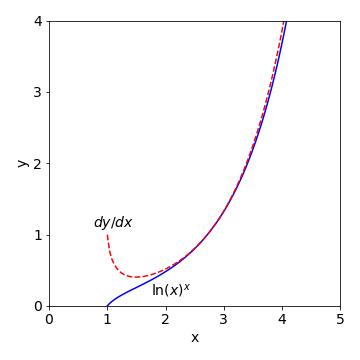
Figure 41: Plot of \((\ln(x))^x\) and its first derivative.

---

(b) The lower curve is the function \(y = (\ln(x))^x\) and when \(x = 1, \,y = 0\) because \(\ln(1) = 0\). When \(x \lt 1,\, \ln(x)\) is negative and raising a negative number to fractional power produces a complex number and which cannot be plotted on these axes; for example \(\ln(-1/2) = i\pi - \ln(2)\).

The derivative is the function \(y\) itself, times a term in \(\ln(\ln(x))\) and \(1/\ln(x)\). When \(x \lt 1\) the derivative is a complex number because it is multiplied by \(y\) which here is the log of a negative number. At \(x\) values just larger than \(1\), the \(1/\ln(x)\) term is large and the derivative is almost 1, but as \(x\) increases that term becomes smaller, but only slowly. The other term \(\ln(\ln(x))\) also increases only slowly with \(x\) and now when combined these two terms are almost constant with a value slightly greater than 1, which is best seen by separately plotting these values. Therefore, the derivative closely follows the value of \(y\) when \(x\) is large.

Q20 answer

It is easier to rewrite the function as \(f = y(s)h(s)\) and then write the product rule, equation (19), as

\[\displaystyle \frac{df}{ds}=y\frac{dh}{ds}+h\frac{dy}{ds}\]

remembering that \(h\) and y are function of \(s\). The derivative \(dh/ds\) is needed and as \(\displaystyle h(s)=e^{ax(s)}\) therefore

\[\displaystyle \frac{dh(s)}{ds}=-a\frac{dx}{ds}e^{-ax(s)}\]

The full derivative is

\[\displaystyle \frac{df}{ds}=-ay(s)e^{-ax(s)}\frac{dx(s)}{ds}+e^{-ax(s)}\frac{dy(s)}{ds}\]

The same result is obtained by SymPy as shown next.

a, s, x, y, f = symbols('a, s, x, y, f')
y = Function('y')
x = Function('x')
f = y(s)*exp(-a*x(s))
ans = diff(f,s)
simplify(ans)

Q21 answer

(a) Differentiating using the product rule produces,

\[\displaystyle y'\equiv \frac{dy}{dx}=nx^{n-1}\ln(x)+x^{n-1}\]

Next, multiply both sides by \(x\) then substitute \(y = x^n\ln(x)\) to obtain \(xy′ = ny + x^n\).

(b) There are two ways of calculating \(y''\); either differentiate the last answer or do the calculation directly. Differentiating the last result produces

\[\displaystyle xy''+y'=ny'+nx^{n-1}\]

and rearranged this is \(\displaystyle xy''=(n-1)y'+nx^{n-1}\).

Differentiating directly is a little more difficult

\[\displaystyle \frac{d^2y}{dx^2}=\frac{d}{dx}\left( nx^{n-1}\ln(x)+x^{n-1}\right)=n(n-1)x^{n-2}\ln(x)+nx^{n-2}+(n-1)x^{n-2}\]

Multiplying by \(x\) and simplifying gives

\[\displaystyle xy'' = (n - 1)nx^{n-1} \ln(x) + nx^{n-1} + (n - 1)x^{n-1}\]

Next, substituting

\[\displaystyle nx^{n-1}\ln(x) = y′ - x^{n-1}\]

and simplifying produces

\[\displaystyle xy′′ = (n - 1)y′ + nx^{n-1}\]

If you do this calculation with SymPy the derivatives can easily be simplified as shown below.

x,y,n = symbols('x, y, n')
ans = simplify(diff(x**n*ln(x),x)  )   # 1st derivative
ans

simplify(diff(ans,x) )               # second derivative

Q22 answer

Velocity is distance per unit time and is defined as \(\displaystyle \frac{dx}{dt}= v\) , and therefore \(\displaystyle \frac{d^2x}{dt^2}=\frac{dv}{dt}\).

To change the differentiation variable from \(t\) to \(x\) use the function of function method, equation, (22) written as \(\displaystyle \frac{dv}{dt}=\frac{dv}{dx}\frac{dx}{dt}\).

The result is

\[\displaystyle \frac{d^2x}{dt^2}=\frac{dv}{dt}=\frac{dv}{dx}\frac{dx}{dt}=\frac{dv}{dx}v\]

Because

\[\displaystyle \frac{d}{dx}\left(\frac{v^2}{2} \right) =v\frac{dv}{dx}\]

by comparing the last two results it follows that

\[\displaystyle \frac{d}{dx}\left(\frac{v^2}{2} \right)=\frac{d^2x}{dt^2}\]

an equation that is important in dynamics.

Q23 answer

Differentiating both sides of the equation with respect to \(x\) gives,

\[\displaystyle 2(x^2+y^2)\left(2x+2y\frac{dy}{dx} \right)=a^2\left(2y\frac{dy}{dx}-2x \right)\]

and simplifying gives

\[\displaystyle \frac{dy}{dx}=-\frac{x}{y}\frac{\left(2(x^2+y^2)+a^2\right)}{\left(2(x^2+y^2)-a^2\right)}\]

By solving this last equation when \(dy/dx=0\) the coordinates where the gradient is zero can be found. One obvious condition is when \(x = 0\) then \(y = \pm a\). Next, setting the top square bracket to zero, produces \(y=\sqrt{-a^2/2-x^2}\) which has to be a complex number and does not appear to lie on our curve.

(c) A change in coordinates from Cartesian to plane polar coordinates means using \((r,\, \theta)\) instead of \((x,\, y)\) to define the curve as shown in Fig. 7. The new coordinate \(r\) is the straight line distance from the origin to the curve and by Pythagoras’ theorem, \(r^2 = x^2 + y^2\). The polar angle is \(\theta\) and is conventionally chosen to be the angle anti-clockwise away from the horizontal axis. This angle is calculated using either \(\cos(\theta) = x/r\), or \(\sin(\theta) = y/r\). Changing the lemniscate into polar coordinates can be done in two steps, the first of which uses the trigonometric identity

\[\displaystyle \cos^2(\theta) - \sin^2(\theta) = \cos(2\theta)\]

First, calculate \(y^2 - x^2\) using the definitions of sine and cosine

\[\displaystyle y^2-x^2=r^2\left(\cos^2(\theta)-\sin^2(\theta)\right)=-r^2\cos(2\theta)\]

Second, substituting into \((x^2 + y^2)^2 = a^2(y^2 - x^2)\) produces

\[\displaystyle r^2 = -a^2\cos(2\theta) = +a^2\cos(2\theta)\]

which is the lemniscate equation in polar coordinates. The gradient is \(dr/d\theta\), therefore

\[\displaystyle r\frac{dr}{d\theta}=-2a^2\sin(2\theta)\qquad \text{or}\qquad \frac{dr}{d\theta}=\frac{2a\sin(2\theta)}{\sqrt{\cos(\pi-2\theta)}}\]

The maximum and minimum occur when the derivative is zero, which occurs at \(\theta = 0^\text{o}\) or \(180^\text{o}\) respectively. When \(\theta\) is zero then \(r = \pm a\), but \(r\) is always positive, and so this gives the maximum, see Fig. 7. When \(\theta = 45^\text{o}\), the curve has its minimum at the origin because \(r = 0\). The maximum gradient of infinity, occurs when \(dx/dy = 0\) which it does when \(\theta = \pm \pi/3\) and \(\theta = \pm 2\pi /3\).

Q24 answer

(a) Differentiating once gives \(\displaystyle \frac{d}{dx}e^{ax^2+x}=e^{ax^2+x}(2ax+1)\)

and again produces

\[\displaystyle \frac{d^2}{dx^2}e^{ax^2+x}=\frac{d}{dx}e^{ax^2+x}(2ax+1)=e^{ax^2+x}\left((2ax+1)^2+2a \right)\]

(b) Differentiating gives \(\displaystyle \frac{d}{dx}\ln(ax+b)^2=2a\frac{\ln(ax+b}{ax+b}\)

and again produces

\[\displaystyle 2a\frac{d}{dx}\frac{\ln(ax+b}{ax+b}=\frac{2a^2}{(ax+b)^2}-\frac{2a^2\ln(ax+b)}{(ax+b)^2}\]

which can clearly be simplified.

Q25 answer

As \(y=\sqrt{a^2-x^2}\), differentiating once and twice gives \(\displaystyle \frac{dy}{dx}=-x(a^2-x^2)^{-1/2}\) and \(\displaystyle \frac{d^2y}{dx^2}=-(a^2-x^2)^{-1/2}-x^2(a^2-x^2)^{-3/2}\).

By substituting and rearranging

\[\displaystyle \frac{d^2y}{dx^2}=\frac{dy}{dx}\left(\frac{1}{x}+\frac{x}{y^2} \right)\]

therefore

\[\displaystyle \frac{d^2y}{dx^2}=\frac{a^2}{xy^2}\frac{dy}{dx}\]

which is

\[\displaystyle y''=\frac{a^2}{xy^2}y'\]

because \(y^2+x^2 = a^2\).

Alternatively, starting with the first equation as given in the question, the derivatives are

\[\displaystyle y\frac{dy}{dx}=-x\quad \text{ and }\quad \displaystyle \left(\frac{dy}{dx} \right)^2+y\frac{dy}{dx}=-1\]

because the derivative of \(y\) is \(dy/dx\). Substituting for \(y\) and rearranging produces the same answer.

Q26 answer

Differentiating twice gives \(\displaystyle \frac{d^2}{dx^2}f(x)=\frac{d}{dx}f(x)=f(x)\) and by induction therefore \(\displaystyle \frac{d^n}{dx^n}f(x)=f(x)\).

From the information given in the question it follows that \(\displaystyle \frac{d^n}{dx^n}f(0)=f(0)=1\). As the Maclaurin expansion of \(f\) is

\[\displaystyle f(x)=f(0)+f'(0)x+f''(0)\frac{x^2}{2!}+ f'''(0)\frac{x^3}{3!}+\cdots\]

because each derivative is unity the series is

\[\displaystyle f(x)=1+x+\frac{x^2}{2!}+\frac{x^3}{3!}+\cdots+ =e^x\]

and the function is the exponential as you may have guessed from the question.

Q27 answer

If \(u=dx/dt\),differentiation with respect to \(t\) gives \(\displaystyle \frac{du}{dt}=\frac{d}{dt}\left( \frac{dx}{dt}\right) =\frac{d^2x}{dt^2}\).

On the left of the equation

\[\displaystyle u\frac{du}{dx}=\frac{dx}{dt}\frac{d}{dx}\left( \frac{dx}{dt} \right)=\frac{dx}{dt}\frac{d^2x}{dxdt}=\frac{d^2x}{dt^2}\]

which is the same result, and the relationship is verified. Notice that in this last calculation \(d/dx\) operates on\( dx/dt\) before the \(dx\) are cancelled.

Q28 answer

(a) Differentiating with respect to \(q\), gives \(\displaystyle (1-q^2)N\frac{d}{dq}f(qN)-2qf(qN)+N\ln(q)+N=0\)

(b) and with respect to \(N\) gives, \(\displaystyle (1-q^2)N\frac{d}{dN}f(qN)+q\ln(q)=0\)

Q29 answer

(a) By direct differentiation \(\displaystyle nx^{n-1} + ny^{n-1} \frac{dy}{dx} = 0\). Rearranging gives \(\displaystyle \frac{dy}{dx}=-\frac{x^{n-1}}{y^{n-1}}\) which is the answer sought.

(b) If you cannot remember the differential of tan, convert it into \(\sin()/\cos()\) then the equation becomes \(\displaystyle \frac{\sin(y)}{\cos(y)} = \sinh(x)\).

Differentiating both sides gives

\[\displaystyle \frac{\cos(y)}{\cos(y)}\frac{dy}{dx}+\frac{\sin^2(y)}{\cos^2(y)}\frac{dy}{dx}=\cosh(x); \qquad \frac{dy}{dx}=\cosh(x)\cos^2(y)\]

The second derivative is \(\displaystyle \frac{d^2y}{dx^2}=\sinh(x)\cos^2(y)-2\cosh(x)\cos(y)\sin(y)\frac{dy}{dx}\) which can be simplified a little further.

Q30 answer

Both \(V\) and \(\psi\) are functions of \(x\). Operating once with \(D\) is formally

\[-D(D^2\psi) + D(V\psi) = ED\psi\]

and using the product rule gives

\[-D^3\psi+\psi DV+VD\psi =ED\psi\]

and differentiating again by left-multiplying with \(D\)

\[\displaystyle -D^4\psi + D(\psi DV + VD\psi) = ED^2\psi\]

\[\displaystyle -D^4\psi + (D\psi)(DV) + \psi D^2V + (DV)(D\psi) + VD^2\psi = ED^2\psi \]

then left multiplying by \(\psi\) and rearranging

\[\displaystyle \psi D^4\psi=2\psi (D\psi)(DV)+\psi^2 D^2V+(V-E) D^2\psi^2\]

which looks somewhat like the answer needed but the first and second terms are different. As the answer required is given we can see if this is correct by expanding \(D(\psi^2DV)\) which gives

\[D(\psi^2DV) = 2\psi(D\psi)(DV) + \psi^2D^2V\]

therefore the relationship is verified.

In common notation this last equation is \(\displaystyle \frac{d}{dx}\left( \psi^2\frac{dV}{dx}\right)=2\psi\frac{d\psi}{dx}\frac{dV}{dx}+\psi^2\frac{d^2V}{dx^2}\).

Q31 answer

(a) The slope at point \(T\) is \(\displaystyle \frac{dy}{dx}=\frac{1}{t}\). The equation of the tangent line at any point is \(y - 2at = (x - at^2)/t\).

(b) The point \(P\) is at \(y=0\) therefore is at \((at^2,0)\). Point F is at \((a,0)\) therefore the length PF is \(a+at^2\). Point T has coordinates \((at^2 , 2at)\) and by Pythagoras’ theorem the distance FT is

\[\displaystyle \sqrt{(at^2-a)^2+(2at)^2} =a^2(t^4+2t^2+1)=a+at^2\]

The distances FP and FT are equal, therefore the triangle FPT is isosceles, and because the ray into the parabolic mirror is parallel to the x-axis, the angle PTF = FPT.

This construction proves that all rays travelling parallel to the parabola’s axis pass through the focus, because T could be any point on the parabola and FP and FT are always equal to one another. Because all rays originating at infinity are parallel to one another and parallel to the axis of the parabola, on entering the parabola they will each pass through the focus. If a mirror with a spherical surface is used, then not all rays pass through the same point and an aberrated focus will be formed.

Q32 answer

(a) The units are number/mole \(\cdot\) J s \(\cdot\,\mathrm{ s^{-1}}\) which is energy/mole. The first term is the zero point energy because it is a constant and does not depend on the vibrational frequency.

(b, c) Differentiating \(U\) with respect to \(T\) is done inside the integral, because the integrand depends on \(T\), and gives,

\[\begin{split}\displaystyle \begin{align}C_v&=\frac{dU}{dT}=\frac{9Nh}{\nu_D^3}\int_0^{\nu_D}\nu^3\frac{d}{dT}\left( \frac{1}{e^{h\nu/k_BT} -1} \right) d\nu\\&= \frac{9Nh^2}{\nu_D^3k_BT^2}\int_0^{\nu_D}\nu^4\frac{e^{h\nu/k_BT}}{(e^{h\nu/k_BT}-1)^2} d\nu \end{align}\end{split}\]

Substituting \(x = h\nu/k_BT\), which is dimensionless, and \(\theta = h\nu_D/k_B\), which has units of K and is called the Debye temperature, and rearranging with \(dx = (h/k_BT)d\nu\), gives

\[\begin{split}\displaystyle \begin{align}C_V&=\frac{9Nh^2}{k_BT^2}\left(\frac{h}{\theta k_B} \right)^3\left(\frac{k_BT}{h} \right)^5\int_0^{\theta/T}x^4\frac{e^{x}}{(e^{x}-1)^2} dx \\&=9Nk_B\left(\frac{T}{\theta } \right)^3 \int_0^{\theta/T}\frac{x^4e^{x}}{(e^{x}-1)^2} dx\end{align}\end{split}\]

The limits are converted into dimensionless units also. The heat capacity has units of J/ K determined by \(Nk_B\) because \(x\) is dimensionless.

(d) At low temperatures the upper limit \(\theta/T \to \infty\) can be safely assumed and the integral is

\[\displaystyle C_{V,T\to \infty}=9Nk_B\left(\frac{T}{\theta } \right)^3 \int_0^{\infty} \frac{ x^4e^{x} }{(e^{x}-1)^2} dx\]

It does not matter whether or not if the integral can be solved analytically or numerically as the result is a constant, thus \(\displaystyle C_{V,T\to \infty} \approx \left( \frac{T}{\theta} \right)^3\) and zero at zero temperature. At low temperatures, the \(T^3\) law is observed experimentally.

At high temperatures, making the upper limit of the integral zero because \(T\) is large and \(\theta/T \to 0\), will yield \(C_V = 0\), because both limits to the integration are then the same. However this does not make sense physically; the crystal must have considerable internal energy which increases with increase in temperature. A more cautious approach to the limit will allow us to expand each exponential because \(x\) is small. The expansion is \(\displaystyle e^x=1+x+\frac{x^2}{2!}+\cdots\) and because \(x^2 \ll x\) the integral need only be expanded to single powers in \(x\);

\[\begin{split}\displaystyle \begin{align}C_{V,T\to \infty}&\approx 9Nk_B\left(\frac{T}{\theta } \right)^3 \int_0^{\infty} \frac{ x^4(1+x+\cdots) }{x^2} dx\\&=9Nk_B\left(\frac{T}{\theta } \right)^3 \int_0^{\infty} x^2 dx\\&= 3Nk_B\end{align}\end{split}\]

The heat capacity at high temperature is the same as predicted and close to the \(3R\)/mole that is observed experimentally, \(R\) being the ideal gas constant.

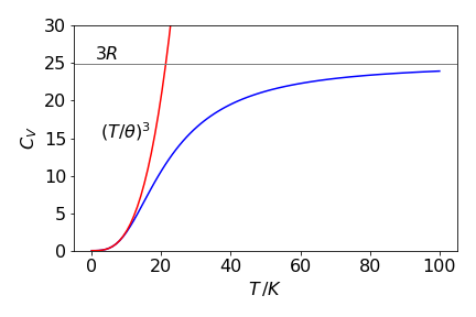
Figure 41a. Heat capacity vs temperature with a Debye temperature \(\theta\) for potassium of \(41.5\) K . Also shown is the high and low temperature behaviour.

---

Q33 answer

Differentiating [B] by changing the proton concentration to pH via \(\text{pH} = -\log_{10}(\text{[H}^+])\) is one approach but it is easier to use the product rule and write

\[\displaystyle \beta=\frac{d[\text{B}]}{d[\text{H}^+]}\frac{d[\text{H}^+]}{d\text{pH}}\]

Differentiating the pH equation (effectively \(x = -\log_{10}(y)\)) gives

\[\displaystyle -\frac{1}{[\text{H}^+]\ln(10)}\frac{d[\text{H}^+]}{d\text{pH}}=1\]

and

\[\displaystyle \frac{d[B]}{d[\text{H}^+]}=-\frac{K_w}{[\text{H}^+]^2}-1-\frac{C_BK_a}{ ([\text{H}^+]+K_a)^2 }\]

giving

\[\displaystyle \beta=2.303\left(\frac{K_w}{[\text{H}^+]}+[\text{H}^+]+\frac{C_BK_a[\text{H}^+]}{ ([\text{H}^+]+K_a)^2 } \right)\]

The calculation is also easy using SymPy.

CB, Kw,Ka,H,pH = symbols('CB, Kw, Ka, H, pH')

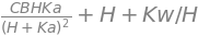
B =  Kw/H-H+CB*Ka/(Ka+H)
pH= -log(H)
ans= diff(B,H)/diff(pH,H)
simplify(ans)

(b) Plotting \(\beta\) produces the graph below where the buffer capacity is a maximum just above pH = 4 which is close to the value of the p\(K_a\). The width of the peak demonstrates the ability of the buffer to resist changes in pH. The total base concentration is \(0.02\) M.

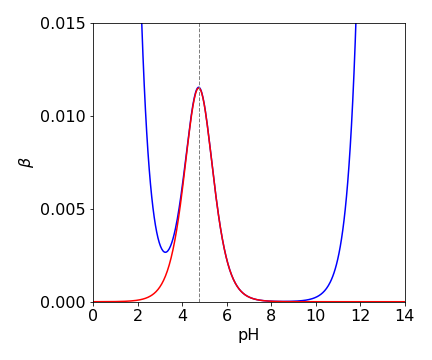
Figure 42. Buffer capacity vs pH where \(K_a=10^{-4.2}\) shown as a dashed line.

---

(c) The maximum or minimum \(\beta\) occurs at

\[\displaystyle \frac{d\beta}{d[\text{H}^+]}=2.303\left(-\frac{K_w}{[\text{H}^+]^2}+1+\frac{C_BK_a}{ ([\text{H}^+]+K_a)^2 } -2\frac{C_BK_a[\text{H}^+]}{ ([\text{H}^+]+K_a)^3 } \right)=0\]

which simplifies to

\[\displaystyle ([\text{H}^+]+K_a)^3\left( 1-\frac{k_w}{[\text{H}^+]^2} \right) +C_BK_a(K_a-[\text{H}^+])=0\]

The minimum occurs when \(K_w \approx [\text{H}^+]^2\) or at pH \(\approx 8\), as here the first term is zero and the second term is also small \(\approx C_BK_a^2\) or \(\approx 10^{-10}\) and will not change the minimum by much.

In acid solution, \(K_w /[\text{H}^+]^2 \ll 1\) and can be ignored compared to unity, hence

\[\displaystyle (\;[\text{H}^+]+K_A)^3 + C_BK_a(K_a-[\text{H}^+]\;)=0\]

which is still hard to solve, but it can be done by the Newton-Raphson method, Section 10. Only the term in \(C_B\) can contribute to the buffering (as the cubic term is small and can be ignored) and give rise to the maximum. . The result shows that, to a good approximation, \(K_a = [\text{H}^+]\). The calculation using a built-in function is as follows, with buffer concentration as \(0.01\) molar.

Ka = 10**(-4.2)
CB = 0.01
Kw = 1e-14
f01= lambda H: (H+Ka)**3*(1-Kw/H**2)+CB*Ka*(Ka-H)
ans= fsolve(f01, 1.0e-7)
print('{:s} {:6.3g} {:s} {:6.3g}'.format( 'Ka =', Ka,' H+ =', float(ans) ))  

Ka = 6.31e-05  H+ = 6.65e-05

Q34 answer

(a) As velocity \(v\) is distance/time, velocity \(v(t)=dy/dt\) and as \(y\) is expressed a a log it is convenient to use the general form

\[\displaystyle \frac{d\ln(f(x))}{dt}\equiv\frac{1}{f(x)}\frac{df(x)}{dt}\]

which gives

\[\displaystyle v(t)=\frac{dy}{dt}=ab\frac{e^{2bt}-1}{e^{2bt}+1}\]

(This may also be expressed as \(ab/\tanh(bt)\)). When enough time has elapsed \(2bt\) is large and the exponential terms become far greater than either \(+1\) or \(-1\) making these unimportant. The exponential terms can now be cancelled leaving the terminal velocity as \(ab\) or \(\displaystyle 2\sqrt{\frac{gm}{\rho CA}}\).

(b,c) Using the values given in the question,the terminal velocity of the skydiver is \(\approx 53\) m/s (\(118.5\) mph) compared to \(28\) m/s for a hailstone. No wonder they hurt so much when they strike you! The speed of the hailstone is surprisingly fast for its small mass, but its area is also very small and therefore so is its air resistance. If there were no air resistance, both bodies would fall at the same speed at all times and this would reach \(gt\) at time \(t\) if they were both initially at rest.

The energy a hailstone contains is \(0.77\) J; the skydiver \(98.3\) kJ. The kinetic energy at terminal velocity is \(\displaystyle \frac{mv^2}{2}=\frac{gm^2}{\rho CA}\) and inversely proportional to area. The skydiver has an area 1.5 m\(^2\) the hailstone \(3.14 \cdot 10^{-4} \,\mathrm{m^2}\). Incidentally, you can see that if the skydiver doubles their surface area then the speed is reduced only as \(\sqrt{2}\) and hence you can understand why a parachute has to be so large.

To find the \(95\)% time for the skydiver \(\displaystyle \frac{e^{2bt}-1}{e^{2bt}+1}=0.95\) has to be solved for \(t\) with \(\displaystyle b=\sqrt{\frac{g\rho C A}{m}} = 0.368\). SymPy could be used but it is just as easy to rearrange the equation into \(\displaystyle e^{2bt}=39\) and taking logs. The time taken to reach \(95\)% of terminal velocity is \(\approx 5\) s and the distance travelled is \(169\) m.

(d) Using the formula for the terminal velocity the cat is supposedly able to produce a surface area of \(3\,\mathrm{ m^2}\) by spreading out its legs. This is such a large area compared to the skydiver (\(1.5\,\mathrm{ m^2}\)), one has to presume that the fur also adds considerably to the air resistance, and so it is the area times \(C\), the air-drag coefficient, that is larger, not just the area itself. Therefore \(AC \approx 1.5\) for the cat and \(0.75\) for the skydiver.

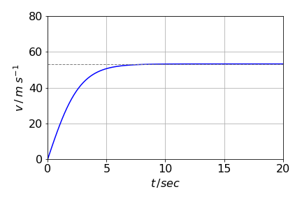
Figure 43. Velocity (m/s) vs time in seconds for the skydiver. The acceleration to terminal velocity is rather rapid and is reached in as little as \(\approx 7\) seconds. The dashed line shows the terminal velocity.

---

Q35 answer

Differentiating \(e^{\alpha x}\) once produces \(\displaystyle \frac{d}{dx}e^{\alpha x}=\alpha e^{\alpha x}\) and so \(n\) times over \(\displaystyle \frac{d^n}{dx^n}e^{\alpha x}=\alpha ^ne^{\alpha x}\). Notice that the result has the characteristic form \(H\psi = E\psi\), if the eigenvalue is \(E = \alpha^n\) and the wavefunction \(\psi=e^{\alpha x}\).

(b) Repeating the calculation with \(\sin(\alpha x)\) produces

\[\displaystyle \frac{d^n}{dx^n}=\sin(\alpha x)=\alpha^n\sin(\alpha x)\]

but this is an eigenvalue - eigenvector equation only when \(n\) is even. When \(n\) is odd,

\[\displaystyle \frac{d}{dx}=\sin(\alpha x)=\alpha\cos(\alpha x)\]

which is not an eigenvalue - eigenvector equation. However, the function \(\sin(\alpha x)\) is a solution to the particle in a box problem because, in the Schroedinger equation, the operator representing kinetic energy is always present with \(n\) = 2 as kinetic energy is present as the second derivative.

In quantum mechanics the momentum operator

\[p=\displaystyle -i\hbar\frac{d}{dx}\]

and as kinetic energy is \(\displaystyle \frac{p^2}{2m}\) therefore

\[\displaystyle \frac{1}{2m}\left(-i\hbar\frac{d}{dx} \right)^2=-\frac{\hbar^2}{2m}\frac{d^2}{dx^2}\]

Q36 answer

Substituting for \(E\) and after rearranging

\[\displaystyle -\frac{\hbar^2}{2m}\psi^{''}+\left(\frac{kx^2}{2}-\frac{3}{2}\hbar\left( \frac{k}{\mu} \right)^{1/2} \right)\psi=0\]

Next differentiate \(\psi\) once and twice, remembering that \( \alpha \) is a constant produces

\[\displaystyle \frac{d\psi}{dx}=\left( \frac{4\alpha^3}{\pi} \right)^{1/4} \left( e^{-(\alpha /2)x^2} -\alpha x^2 e^{-(\alpha/2)x^2} \right) \]

\[\displaystyle \frac{d^2\psi}{dx^2}=\left( \frac{4\alpha^3}{\pi} \right)^{1/4} \left(-3+\alpha x^2 \right)\alpha x e^{-(\alpha/2)x^2} \]

Next, multiply by \(\displaystyle -\frac{\hbar^2}{2m}\) and add \(\displaystyle\left(\frac{kx^2}{2}-\frac{3}{2}\hbar\sqrt{\frac{k}{\mu}} \right)\psi\) to complete the equation. This produces

\[\displaystyle -\frac{\hbar^2}{2\mu}\left( \frac{4\alpha^3}{\pi} \right)^{1/4} \left(-3+\alpha x^2 \right)\alpha x e^{-(\alpha/2)x^2}+\left( \frac{kx^2}{2} -\frac{3\hbar}{2}\sqrt{\frac{k}{\mu}}\right)\left(\frac{4\alpha^3}{\pi} \right)^{1/4}xe^{-(\alpha /2)x^2}=0 \]

If the left-hand side of this horrid equation can be simplified to make zero, this will show that \(\psi\) is a solution of the equation.

Assuming that this equation is zero and that \(\psi\) is a solution,then most of the constants and the exponential terms can now be divided away to leave,

\[\displaystyle -\frac{\hbar^2}{2\mu} \left(-3+\alpha x^2 \right)\alpha +\left( \frac{kx^2}{2} -\frac{3\hbar}{2}\sqrt{\frac{k}{\mu}}\right)=0 \]

Only the constant \(\alpha\) remains and must be replaced with the expression given in the question; substituting \(\displaystyle \alpha=\sqrt{\frac{\mu k}{\hbar^2}}\) produces

\[\displaystyle -\frac{\hbar^2}{2\mu} \left(-3+\sqrt{\frac{\mu k}{\hbar^2}} x^2 \right)\sqrt{\frac{\mu k}{\hbar^2}} +\left( \frac{kx^2}{2} -\frac{3\hbar}{2}\sqrt{\frac{k}{\mu}}\right)=0 \]

After expanding and cancelling terms this expression does become zero and therefore

\[\displaystyle \psi = 2\sqrt{2}\left(\frac{\alpha ^3}{\pi} \right)^{1/4}xe^{-(\alpha /2)x^2}\]

is the harmonic oscillator wavefunction for \(\nu\)=1 and its energy is

\[\displaystyle E= \frac{3}{2}\hbar\sqrt{\frac{k}{\mu}}\]

Using Sympy a result of zero is produced after some more simplification that the programme fails to do unless the instruction \(\mathtt{,positive =True}\) is added to the first line as an argument to \(\mathtt{symbols}\).

psi,x,hbar,E,k,alpha,mu = symbols('psi, x, hbar, E, k, alpha, mu ') # to get zero add ..' ,positive=True)

alpha = sqrt(mu*k/hbar**2)

E = (3/2)*hbar*sqrt(k/mu)

psi = lambda x: sqrt(sqrt(4*alpha**3/pi))*x*exp(-(alpha/2)*x**2)

eqn = ( (-hbar**2/(2*mu))*diff(psi(x),x,x) +((1/2)*k*x**2-E)*psi(x)) 
 
simplify((eqn) )

Q37 answer

Differentiation gives

\[\displaystyle \frac{dE}{dn}=\hbar\omega_e -2\hbar x_e\omega_e(n+\frac{1}{2})\]

and therefore

\[\omega = \omega_e-2 x_e\omega_e(n+1/2)\]

Rearranging to find \(n+1/2\) and then substituting into the energy \(E\), which will eliminate \(n\), produces

\[\displaystyle E=\frac{\hbar}{2x_e}(\omega_e-\omega)-\frac{\hbar}{4\omega_e}(\omega_e-\omega)^2\]

Rearranging gives

\[\displaystyle \omega^2 =\omega_e^2=4x_e\omega_e \frac{E}{\hbar}\]

where \(E\) is the energy in the potential well. In an optical experiment this is the energy of the photon \(E_{h\nu} \equiv E_{\hbar\omega}\) less the zero point energy \(E_0\) of the transition, therefore, \(\omega^2 =\omega_e^2=4x_e\omega_e (E_{\hbar\omega}-E_0)\).

Q38 answer

(a) \(\displaystyle \frac{dV}{dx}=\pi x^2\tan^2(\alpha)\) where 0\(\le x\le h\) and this is the surface area of the cone as it is proportional to \(x^2\). When a volume is differentiated, an area is produced because the dimension is reduced. This function represents how the volume in the cone changes with height and would usually be described as the rate of change of volume with height.

(b) The rate of liquid loss is given as \(5\,\mathrm{ cm^3\, min^{-1}}\) and this is \(dV/dt\) where \(V\) is the volume; however, only \(dV/dx\) has been calculated. These two derivatives are connected with the ‘function of a function’ equation

\[\displaystyle \frac{dV}{dt}=\frac{dV}{dx}\frac{dx}{dt}\]

where \(dV/dt\) is the rate of decrease of the liquid’s volume. Rearranging to \(\displaystyle \frac{dx}{dt}=\frac{dV}{dt}/\frac{dV}{dx}\) and from the values given \(\displaystyle \frac{dx}{dt}=\frac{5}{\pi x^2}\tan^2(\alpha)\) and when \(x = 2\) and as \(b\) = 3 and \(h = 9\) cm, \(\tan(\alpha) = 1/3\), and the rate of liquid level decrease is \(3.6\,\mathrm{ cm \,min^{-1}}\) which clearly increases as \(x\) decreases because the volume flow rate is a constant.

Q39 answer

(a) Starting with the harmonic potential, the first derivative is \(\displaystyle \frac{dV_{HO}}{dr}=2k(r-r_e)\) and the second derivative \(\displaystyle \frac{d^2V_{HO}}{dr^2}=2k\). The radius of curvature is

\[\displaystyle \rho=\frac{\left( 1+4k^2(r-r_e )\right)^{3/2}}{2k}\]

and when \(r=r_e\) the curvature is \(\rho_{r_e}=1/2k\).

(b) The Morse potential calculation is effectively the same but more involved and is done using Sympy as follows,

Vm,De,r,re,beta,V,k=symbols('Vm, De, r, re, beta, V, k')

Vm = De*(1 - exp(-(r-re)*beta))**2             # Morse potential

ans= ( 1 + (diff(Vm,r))**2)**(3/2)/( diff(Vm,r,r) )
simplify(ans)

Substituting \(r = r_e\) (and using \(e^0=1\)) into this complex result produces considerable simplification making radius of curvature \(\displaystyle \rho=\frac{1}{2D_e\beta^2}\). Sympy also finds this result.

ans.subs(r,re)

(c) Comparing this last result with that from the harmonic oscillator the force constant \(k = D_e \beta^2\).

(d) The radius of curvature at the minimum has units of metres/ Newton not just metres because the potential energy is plotted on axes of N m \(\equiv\) J vs. m. The constant \(\beta\) has units of m\(^{-1}\) and \(D_e\) units of J so the units of the radius are also m/N for the Morse potential.

The units of the force constant are N/m, the dissociation energy must be in J and \(\beta\) is in \(m^{-1}\) as the exponential in which it appears must be dimensionless. Therefore \(k(N/m) = D_e (\text{J}) \beta^2 (\mathrm{m^{-2}}) \equiv \mathrm{J\,m^{-2}} = \mathrm{N\, m\, m^{-2}} =\mathrm{ N\, m^{-1}}\), which is dimensionally correct. A joule is a newton \(\cdot\) metre because energy is force times distance.

Q40 answer

As force is the derivative of the potential with extension and is also defined by Hooke’s law as force constant \(\cdot\) extension. Therefore, the force constant is the second derivative of potential with extension.

If the potential \(V = ks^2/2\) with \(s\) the extension then \(\displaystyle \frac{d^2V}{ds^2}=k\). Differentiating the Morse potential with respect to \(s\) produces the force,

\[\displaystyle \frac{dV_m}{ds}=2\beta e^{-\beta s}D_e\left( 1-e^{-\beta s}\right)\]

and again

\[\displaystyle \frac{d^2V_m}{ds^2}=2\beta^2 D_e(2e^{-\beta s}-1)e^{-\beta s}\]

and at the minimum \(s=0\) giving \(\displaystyle \frac{d^2V_m}{ds^2}=2\beta^2 D_e\). This is therefore the Hooke’s Law force constant if the two second derivatives of \(V_m\) and \(V\) are assumed equal. This answer is slightly different to that of the previous question as different assumptions were made in these two calculations. In that question, it was assumed, without justification, that the curvature was the same for the harmonic and Morse potential at the minimum; in this question, it is argued dimensionally that the force constant is the second derivative of the potential.

Q41 answer

(a) The internal energy is found by substituting for \(Z\) and differentiating \(\ln(Z)\) with \(T\). The three lines below only involve simplification with no calculation;

\[\begin{split}\displaystyle \begin{align} U&=Nk_BT^2\frac{d}{dT}\ln\left( e^{-\theta /2T} \left( 1-e^{-\theta /T }\right)^{-1} \right) \\ &=Nk_BT^2\left[\frac{d}{dT}\ln\left( e^{-\theta /2T}\right) - \frac{d}{dT}\ln \left( 1-e^{-\theta /T }\right) \right] \\ &=Nk_BT^2\left[-\frac{d}{dT}\ln\left(\frac{\theta }{2T}\right) - \frac{d}{dT}\ln \left( 1-e^{-\theta /T }\right) \right] \end{align}\end{split}\]

Now differentiate with \(T\) and simplify the result by multiplying both top and bottom of the expression by \(e^{\theta/T}\),

\[\displaystyle U=Nk_BT^2\left(\frac{\theta}{2T^2}-\frac{-\theta e^{-\theta /T}}{T^2\left(1-e^{-\theta/T} \right)} \right)=Nk_B\theta \left(\frac{1}{2}+\frac{1}{e^{\theta /T} -1} \right)\]

The heat capacity is

\[\displaystyle C_V=\frac{dU}{dT}=Nk_B\frac{\theta^2}{T^2}\frac{e^{\theta/T}}{\left( e^{\theta/T}-1\right)^2}\]

(b) First, calculate the limits to the internal energy. At high temperatures, the exponential terms are small and can be approximated as the series \(e^x = 1 + x + \cdots\); therefore \(\displaystyle U\approx Nk_B\theta \left(\frac{1}{2}+\frac{T}{\theta} \right)\) and, at even higher temperatures, where \(T/\theta \gg 1\), the internal energy increases in direct proportion to the temperature and \(U = Nk_BT\).

This is exactly what would be expected from a molecule with two degrees of freedom; one degree of kinetic energy and one of potential energy from each molecule with each term contributing \(k_BT/2\).

At high temperatures, expanding the exponentials in the equation for heat capacity as \(\theta/T\) is small produces \(\displaystyle C_v \to Nk_B\frac{\theta^2}{T^2}\frac{T^2}{\theta^2}=Nk_B\) and \(Nk_B=R\) the gas constant.

When the temperature is low and tends to zero, \(T/\theta \ll 1\) then \(e^{\theta/T} \to \infty\) and in the expression for the internal energy \(\displaystyle \frac{1}{e^{\theta/t}-1} \to \frac{1}{e^{\theta/T}} \to 0\) producing the limit \(U=N\hbar\omega /2\) which is the zero point energy.

Consider now the heat capacity at low temperatures. Because the exponentials are again large; \(\displaystyle \frac{e^{\theta/T}}{\left(e^{\theta/T}-1 \right)^2}\to \frac{e^{\theta/T}}{e^{2\theta/T}}=\frac{1}{e^{\theta/T}}\) and therefore \(\displaystyle C_V=Nk_B\frac{\theta^2}{T^2}\frac{1}{e^{\theta/T}}\) and hence \(C_V \to 0\) at \(T \to 0\) because the exponential approaches zero faster than \(1/T^2\) approaches infinity.

(c) Plots of the internal energy and heat capacity are shown in Fig. 44 in reduced units of \(T/\theta\) and ordinates of \(U\) divided by \(Nk_B\theta\) and \(C_V\) by \(Nk_B\). These plots are universal and therefore true for any parameter values because they are in reduced or dimensionless units. The value of \(\theta =\hbar\omega/k_B \equiv h\nu/k_B\) is a few hundred degrees Kelvin; for iodine molecules this is \(127/0.63= 201.6\) K where the vibrational frequency is \(127\,\mathrm{ cm^{-1}}\).

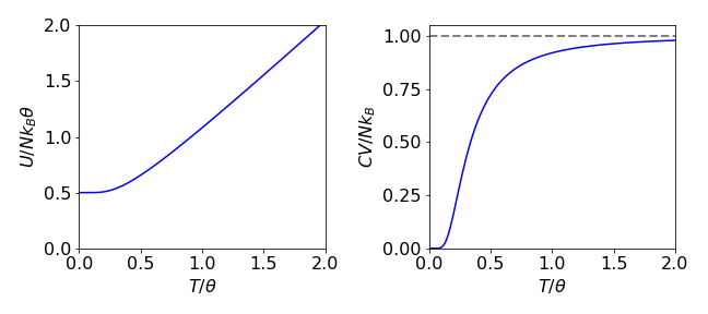
Figure 44. Plots of internal energy and heat capacity in ‘dimensionless’ units. Internal energy is divided by \(Nk_B\theta\) vs \(T/\theta\) and the heat capacity is divided by \(Nk_B\).

---

Q42 answer

The partition function is the sum of the Boltzmann factors for each energy level and is

\[\displaystyle Z=e^{-\gamma \hbar B_0/k_B T} + 1+ e^{+\gamma \hbar B_0/k_B T}\]

where the middle term is unit because \(e^0=1\). Because the derivative used to calculate \(U\) is with respect to \(\beta = 1/k_BT\), this should be substituted for first then replaced after the calculation if necessary; viz; $\(\displaystyle Z = e^{-\gamma \hbar B_0\beta} + 1 + e^{+\gamma \hbar B_0\beta}\)$

(a) Average energy:by direct differentiation with \(\beta\) using the rules for log differentiation,\( \displaystyle \frac{d}{dx}\ln(f(x))=\frac{f'(x)}{f(x)}\) produces

\[\displaystyle U=-N\frac{d}{d\beta}\ln\left(e^{-\gamma \hbar B_0\beta} + 1 + e^{+\gamma \hbar B_0\beta} \right)=-\gamma\hbar B_0N \frac{-e^{-\gamma \hbar B_0\beta} + e^{+\gamma \hbar B_0\beta}}{e^{-\gamma \hbar B_0\beta} + 1 + e^{+\gamma \hbar B_0\beta}}\]

(b) Next,this equation is examined at high and low temperatures to see what form it takes. When \(\beta\) is small (high temperature) by letting \(\beta \to 0\) each exponential can be expanded term by term, since \(\displaystyle e^{\pm x} = 1 \pm x \cdots\), to give

\[\displaystyle U_{high \; T}=-\gamma \hbar B_0 N\frac{-1+\gamma \hbar B_0\beta+1+\gamma \hbar B_0\beta}{1-\gamma \hbar B_0\beta+1+1+\gamma \hbar B_0\beta} =-\gamma \hbar B_0\frac{2\gamma \hbar B_0\beta}{3} \to 0\]

When \(\beta\) is large which occurs at low temperatures, (\(\beta \to \infty\)), \(U_{low\;T} \to -\gamma\hbar B_0N \) because \(e^{-\gamma \hbar B_0\beta} \to 0\) and the remaining exponential terms are very large \(\gg 1\) and cancel out.

In conclusion, the average energy is predicted to be negative at low temperature, since most spins are in the lowest energy level and tend toward zero as the temperature increases, because spins are more equally distributed amongst all levels.

(b) The heat capacity is most easily calculated by changing to temperature rather than using \(\beta\) as our variable. As \(\beta = 1/k_BT\), using the function-of-function equation \(\displaystyle \frac{dU}{d\beta}=\frac{dU}{dT}\frac{dT}{d\beta}\) the heat capacity is \(\displaystyle C_B=\frac{dU}{dT}=-\frac{1}{k_BT^2}\frac{dU}{d\beta}\).

\[\displaystyle -\frac{1}{k_BT^2}\frac{dU}{d\beta}=N\frac{(\gamma\hbar B_0)^2}{k_BT^2}\left( \frac{e^{-\gamma\hbar B_0\beta}+e^{\gamma\hbar B_0\beta}}{e^{-\gamma\hbar B_0\beta}+1+e^{\gamma\hbar B_0\beta}}-\frac{(-e^{-\gamma\hbar B_0\beta}+e^{\gamma\hbar B_0\beta})^2}{(e^{-\gamma\hbar B_0\beta}+1+e^{\gamma\hbar B_0\beta})^2} \right)\]

This complicated equation can be simplified somewhat; it helps to temporarily substitute \(\gamma\hbar B_0\beta = x\) and note that there is a common term in the denominator; the result remains complicated, however,

\[\displaystyle C_B=N\frac{(\gamma\hbar B_0)^2}{k_BT^2}\frac{e^{-\gamma\hbar B_0/k_BT}+4+e^{\gamma\hbar B_0/k_BT}}{(e^{-\gamma\hbar B_0/k_BT}+1+e^{\gamma\hbar B_0/k_BT})^2}\]

Some authors convert the exponentials to cosh functions which will obviously appear to be a different result.

(c) At high and at low temperatures \(C_B\) has different limits. When \(T\) is small, \(T \to\) 0, the exponential \(e^{a/T} \to \infty\) and \(e^{-a/T} \to 0\) where \(\gamma\hbar B_0/k_B = a\).

The two \(e^{a/T}\) terms are far greater than any constants or \(e^{-a/T}\) and then cancel one another; the result is \(\displaystyle C_B \to \frac{1}{T^2e^{a/T}}\to 0\) and so tends to zero, because the exponential increases more rapidly than the \(T^{-2}\) term as \(T\) approaches zero.

When \(T\) is large, each exponential term tends to unity, \(e^0 = 1\), and so \(C_B \to 0\) because of the \(T^{-2}\) term which remains.

The graph of \(C_B\) vs \(T\) is shown below and confirms the limiting values just estimated. The peak in the heat capacity is called the Schottky anomaly and is useful in determining energy level splitting in rare earth ions and transition metals.

The average energy tends to zero as the temperature rises because almost equal populations of spins occupy levels with energies \(E = -\gamma\hbar B_0,\; E = 0\), and \(E = +\gamma\hbar B_0\). That this occurs at such a low temperature is because the energy gaps between nuclear spin levels in a magnetic field, even one as large as \(14\) T, are tiny. The heat capacity \(C_B\) is the rate of change of internal energy \(U\) with temperature. At low temperatures the slope of \(U\) vs \(T\) is constant, because all the spins are in the lowest level and \(C_B = 0\), and at high temperature, the three levels are almost equally populated, therefore, there is no change with temperature. At intermediate temperatures, the rate of increase of energy is large and thus \(C_B\) is also large because nuclei are excited by thermal energy from the lowest spin state into the two others. The figure show the heat capacity and internal energy.

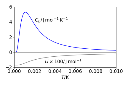
Figure 45 The calculated average energy \(U\) and heat capacity per mole \(C_B\), for the spin 1 nucleus, \(^{14}\)N, in a 14 T magnetic field. The magnetogyric constant \(\gamma \) = 1.47 \(\cdot\) 10⁷ rad /T/s.

---

(d) The entropy is \(\displaystyle S = \frac{U}{T} + Nk_B\ln(Z)\) and using the results already derived,

\[\displaystyle S=-\frac{\gamma\hbar B_0 N}{T}\frac{-e^{-\gamma\hbar B_0/k_BT}+e^{+\gamma\hbar B_0/k_BT} }{e^{-\gamma\hbar B_0/k_BT}+1+ e^{+\gamma\hbar B_0/k_BT}}+Nk_B\ln\left(e^{-\gamma\hbar B_0/k_BT}+1+ e^{+\gamma\hbar B_0/k_BT} \right) \tag{A}\]

This is a rather unforgiving equation and it does not obviously help us to understand the entropy. However, the entropy at high temperature can also be calculated from the equation \(S = k_B\ln(\Omega)\) where \(\Omega\) is the number of microstates. Because there are three states and \(N\) spins that can be in any of these states, then \(\Omega = 3N\), and \(S = Nk_B\ln(3) = 9.13\,\mathrm{ J\, mol^{-1}\, K^{-1}}\).

Evaluating \(S\) using equation A when \(T\) is large, the first term tends to zero, as does the average energy \(U\), and the second term produces \(Nk_B\ln(3)\). The \(\ln(3)\) is produced because at high temperatures the nuclei have an equal chance of taking any of the three orientations to the magnetic field. At low temperatures, only the lowest level is populated so that \(S = Nk_B\ln(1) = 0\) and the nuclear-spin angular momentum points in a direction parallel to the applied field \(B_0\).

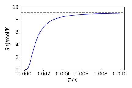
Figure 46. Entropy vs temperature for the three levels spins. The dashed line shows \(S = Nk_B \ln(3)\).