
Solutions Q33 - 44
Contents
Solutions Q33 - 44#
# added here as used later on
%matplotlib inline
import numpy as np
import matplotlib.pyplot as plt
from sympy import *
init_printing()             # allows printing of SymPy results in typeset maths format
plt.rcParams.update({'font.size': 14})  # set font size for plots
Q33 answer#
(a) This expansion needed is \(\displaystyle (1-\alpha)^{-2} = 1=2\alpha +\frac{6}{2!}\alpha ^2 +\frac{12}{3!}\alpha ^3 +\cdots \) and therefore keeping terms only as far as \(\alpha^2\) produces
which simplifies to first order to, \(\displaystyle F= \frac{3k_BT}{2p}\alpha = \frac{3k_BT}{2p}\frac{x}{L}\).
Because the force is proportional to extension \(x\), Hooke’s law is obeyed with the effective force constant \(\displaystyle k=3k_BT/(2pL)\)
(b) Substituting values into the force constant gives \(k\approx 5.6\cdot 10^{-4}\,\mathrm{ N\, m^{-1}}\) for the protein and \(k \approx 1\cdot 10^{-8}\,\mathrm{ N\, m^{-1}}\) for the DNA. Both these force constants are very small compared to those for chemical bonds whose force constants are typically tens to hundreds of \(\mathrm{ N\, m^{-1}}\).
If the protein unfolds after extending by \(28\) nm and if the energy to extend is \(\approx kx^2\), this is \(\approx 4 \cdot 10^{-19}\) J/ molecule. The energy needed for the DNA is about ten times larger; \(\approx 3 \cdot 10^{-18}\) J/molecule. Typical bond dissociation energies are \(300\) kJ/mole or \(4.5 \cdot 10^{-19}\) J/ molecule.
Although the energy input in the protein is comparable to that to dissociating a bond, in the protein this energy is spread over many hundreds of bonds. In this example, those bonds in 28 residues, therefore CC, CN, CH or NH bonds do not break but instead some of the intermolecular and hydrogen bonds do break as the force is applied.
In DNA, the energy input is greater than that needed to break a chemical bond if it were localised. DNA’s vast size on a molecular scale means that there are many more intermolecular interactions than in a protein and therefore, more energy is needed to unfold it. The ‘softness’ of the potential, as reflected in the small force constant, makes this energy less that one might imagine from studying the protein.
The correct energy could be calculated by integrating the force over the extension using the full worm-like-chain equation given above, but this is unhelpful because the force goes to infinity, in a similar manner to that shown in Fig. 29, at full extension. Therefore, we have to assume somewhat arbitrarily, a value of the extension where the protein or DNA unfolds. Experiment shows that this is about \(95\) % of full extension.
Q34 answer#
(a) When \(L/p\) is large,the exponential term tends to zero, so that \(\displaystyle 1-e^{-L/p} \to\) 1 then \(\langle r^2 \rangle \approx 2p(L-p)\). When the polymer contour length is far greater than the persistence length \(\langle r^2 \rangle \approx 2pL\).
(b) When the contour length is smaller than the persistence length, \(L/p \lt\) 1 expanding the exponential gives,
This makes sense as the polymer must be rigid if \(p \gt L\).
Q35 answer#
The Taylor series expansion, equation (17), is made about the separation \(r_e\) at minimum energy. The series produced is
The notation \(U'(r_e)\) and so forth means ‘calculate the derivatives with respect to \(r\) and then evaluate them at \(r_e\)’. The first two derivatives are
and the series is constructed with \(r=r_e\) and is
Notice that the complicated expressions in square brackets are the constants and form the coefficients in the expansion in \((r - r_e)\).
(c) The minimum energy is found at \(r=r_e\) and by substituting into the previous equation this is
Force is the derivative of energy with extension, and has units J/m = N. The extension is \((r-r_e)\) and the first few terms of the derivatives are;
The force constant is therefore \(\displaystyle k=24\epsilon\sigma ^6\left(-\frac{7}{r_e^8}-\frac{26\sigma^6}{r_e^{14}} \right)\) and evaluating with \(\displaystyle r_e = 2^{1/6}\sigma\) produces \(k=36\cdot 2^{2/3} \epsilon/\sigma^2\) which has the correct units of N/m as \(\epsilon\) is energy in joules (\(1\) J \(\equiv 1\) N m), and \(\sigma\) has units of \(\mathrm m^2\). After substituting for \(\sigma\) the first term evaluates to zero.
The vibrational frequency (s\(^{-1}\)) is given by \(\displaystyle \nu=\frac{1}{2\pi}\sqrt k /\mu\) where \(\mu\) is the reduced mass \(\displaystyle \frac{1}{\mu}=\frac{1}{m_1} +\frac{1}{m_2}\) and both atomic masses, \(m_1\) and \(m_2\), are the same for Xe-Xe interaction and \(2.1802 \cdot 10^{-25}\) kg. The frequency produced is \(\nu = 5.18 \cdot 10^{11}\) Hz which is a vibration with a period of \(1.93\) ps and this large value is consistent with a weak intermolecular interaction; the vibrational period for a C-C bond would for example, be very approximately \(100\) times smaller.
(d) A plot of the true and approximate potentials is shown in the next figure; the approximation is parabolic as only terms up to \(\displaystyle (r - r_e )^2 \) are included. Using higher powers in the series improves the approximation to the repulsive potential at small separations, but powers up to at least \(\displaystyle (r-r_e)^{12}\) are needed to fit the attractive part of the potential and even then this is only good from the minimum up to about \(-4\) meV. The 6-12 and the harmonic potential are compared in the figure below.
# L-J 6-12 potential U
sigma   = 389.0      # in pm
epsilon = 20.0e-3    # eV
U  = lambda x: -4.0*epsilon*( (sigma/x)**6 - (sigma/x)**(12) )    # L-J 6-12 potential
numr = 500
r  = np.linspace(0.1,2000,numr)          # make r values 0.1 to 2000, numr values
Ev = [ U(r[i]) for i in range(numr) ]
re = 2**(1/6)*sigma
EH = [36*2**(2.0/3.0)*epsilon/sigma**2*(r[i]-re)**2 - epsilon for i in range(numr)] # harmonic approx

fig1=plt.figure(figsize=(5,5))
plt.rcParams.update({'font.size': 16})  # set font size for plots
plt.plot(r,Ev,color='red',label='L-J 6-12')
plt.plot(r,EH,color='blue',linestyle='dotted',label='Harmonic approx')
plt.axis([300,1200,-1.05*epsilon,1.05*epsilon])
plt.axhline(0,color='gray',linestyle='dashed',linewidth=1)
plt.yticks([-0.02,-0.01,0.0,0.01,0.02])
plt.xlabel('r/ pm')
plt.ylabel('E/ eV')
plt.title('Lennard-Jones 6-12 potential & its aproximation')
plt.legend()
plt.show()
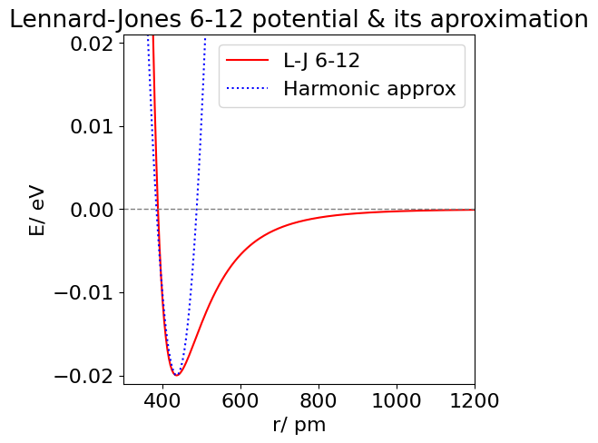
Figure 30. The Lennard-Jones 6-12 potential for Xe (solid) and the harmonic approximation about \(r_e\) (dotted).
Q36 answer#
The sketch, Fig.5, shows that the charges are separated at \(x + d\) for the negative end of the dipole and \(x - d\) for the other. The electric field \(E\) at the ion a distance \(x\) away from the dipole, is force / charge and using equation (29) this is
where, for clarity, \(\beta_0 = 1/(4\pi\epsilon_0 \epsilon)\). Since \(x \gg d \) the two reciprocal terms can be expanded, and from the table of summations, for any general variable \(s\) the series expansions are,
However, our equation must be rearranged into this form by dividing the squared term by \(x\) to give \(1 \pm d/x\). Doing this produces the equation
with \(\beta = \beta_0/d^2 \), moving the constants and expanding using the series above with \(s \equiv d/x \)gives
Canceling terms and rearranging gives,
and as \(x \gg d\) the second term \(d^3/x^5 \) is very small compared to the first and is ignored. The field thus depends on \(x^{-3}\) and this term arises because those in \(x^{-2}\) cancel out leaving only a weaker field in higher powers of the separation. The next figure (below) shows that the approximation to the electric field is good (lower curve) at \(x \gt d\), and was drawn by assuming for simplicity that \(\epsilon \) and the constants \(q/4\pi\epsilon_0 = 1\). In SI units this number should be \(1.44 \cdot 10^{-9}\,\mathrm{ J \,m\, C^{-1}}\). Dielectric constants are dimensionless and for non-polar solvents such as hexane, \(\epsilon \approx 2\) but \(\approx 78\) for polar water; molecular dipoles are typically about \(5\) Debye which is \(16.65 \cdot 10^{-30}\) C m.
The field \(E\) has units force / charge or \(\mathrm{J\, m^{-1}\, C^{-1}}\); the interaction energy is therefore dimensionally field \(\cdot\) charge \(\cdot\) distance, which is force \(\cdot\) distance. Integrating the force from infinity, where it is zero, to a separation \(x\) produces the energy. Using the result for the field the force is first multiplied by the charge \(z\) to give
The interaction energy is the integral of this force and is
and has units \(\displaystyle \mathrm{ \frac{C^2m}{C^2J^{-1}m^{-1}m^2}}=J \).
# energy in reduced units U/(q.beta), and unit charge
# distance is in reduced unit z= x/d; this measures separation in multiples of charge separation d.

E     = lambda z :( -(1+z)**(-2) + (1-z)**(-2)  )
Eapprx= lambda z : 4/z**3
z = np.linspace(1.0001,6.0,100)

fig1=plt.figure(figsize=(5,5))
plt.rcParams.update({'font.size': 16})  # set font size for plots
plt.plot(z, E(z), color='red',label='exact')
plt.plot(z, Eapprx(z), color='blue',label='approx')
plt.axis([1,6,0,4])
plt.ylabel('reduced field '+r'$ E/q\beta$')
plt.xlabel('reduced distance x/d')
plt.title('ion-dipole interaction')
plt.legend()
plt.show()
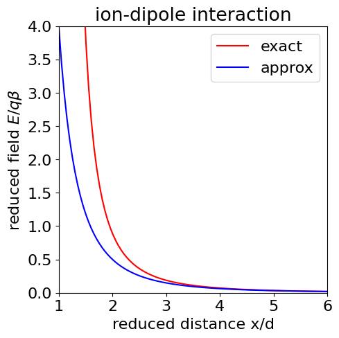
Figure 31. The ion - dipole interaction field \(E\) (in units of \(q\beta/d^2\)) vs reduced separation \(x/d\), top line shows the exact formula, the lower (dash) line shows the approximation \((x/d)^3\) which can be seen only to be good when \(x/d \gt 1\) which in this case means greater than about \(3\).
Q37 answer#
(a) The attractive terms between opposite charges are proportional to \(-(x-d_1)^{-1} - (x-d_2)^{-1}\) and the repulsive terms \(x^{-1} +(x+d_2-d_1)^{-1}\). This leads directly to the equation given in the question, when scaled with the constants needed to put the energy into SI units.
(b) As \(x \gg d\) each term can be expanded using a Taylor series, but to be able to do this properly, each term must be put into the form \(x(1 + d/x)\) and then the condition for series expansion, \(d/x \ll 1\), is produced. The energy is expressed as the sum of attraction and repulsion terms, and after simplifying a little gives,
The series\((1+s)^{-1} =1-s+s^2 -\cdots \) can now be used if \(s\) represents any algebraic expression where \(s \lt 1\), therefore,
where \(\mu _1\) and \(\mu_2\) are the dipole moments \(qd_1\) and \(qd_2\) respectively.
(c) The conversion from units of Debye to J m is \(1\) D \(\equiv 3.33 \cdot 10^{-30}\) C m, the interaction energy of two \(5\) D dipoles at \(2\) nm separation is therefore \(-2\cdot 25 \cdot 3.332 \cdot 10^{-60}/(4\pi 8.854\cdot 10^{-12} \cdot 8\cdot 10^{-27})\) J = \(-6.23 \cdot 10^{-23}\,\mathrm{ J\, molecule^{-1}}\) or \(-0.375\,\mathrm{ kJ\, mole^{-1}}\). At room temperature \(k_BT = 4.14 \cdot 10^{-21}\) J (or \(2.49\, \mathrm{kJ\, mole^{-1} }\)) so at this \(2\) nm separation the dipoles’ alignment is going to be easily disrupted by thermal motion. The thermal energy is really so much larger that no persistent alignment will exist. At \(1\) nm, however, the dipole interaction energy is comparable to thermal energy.
Exercise: Repeat the calculation, supposing that the two dipoles are facing one another parallel and then anti-parallel. A much harder calculation is to calculate the effect of averaging over all angles.
Q38 answer#
(a) The frequency change is shown in the next figure calculated as if the vehicle passes us when standing one metre from the kerb and is traveling at \(60\) mph. Notice that the frequency change is greatest as the vehicle approaches compared to when it moves away. i.e. the curve is not symmetrical.
The relative velocity is calculated by first finding the angle \(\theta\) from the vehicle at \(x\) to the observer at position at \(x_0\), and \(\tan(\theta) = x_0/x\), then finding the projection of this length onto the vehicle’s path via \(\cos(\theta)\).
# Doppler shift

vs  = 330                      # speed of sound m/s
mph = 60                       # vehicle speed in mph
v   = mph *1609.34/3600.0      # mph in m/s
v0  = 0.0                      # observer's speed
x0  = 1.0                      # observer's distance
f0  = 440.0                    # siren's frequency Hz

numx = 200                   # number of data points
x = np.linspace(-10,10,numx) # numx points evenly spaced from -10 to 10
print('{:6.2f} {:s}{:6.2f}{:s} '.format(mph, 'mph is equivalent to ',v,' m/s' ))

f = lambda v, x : f0*(vs+v0)/(vs-v) if x > 0 else f0*(vs+v0)/(vs+v)

rel_v = [ v*np.cos(np.arctan(x0/x[i])) for i in range(numx)]  # angle to observer at x0 then apparent velocity

f01 = [ f( rel_v[i], x[i] ) for i in range(numx)]

fig1 = plt.figure( figsize=(5, 5) )
plt.rcParams.update({'font.size': 16})  # set font size for plots
plt.plot( x, f01,color='blue')
plt.axhline(f0,color='gray',linewidth=1)
plt.axvline(0 ,color='gray',linewidth=1)
plt.xlabel('distance /m')
plt.ylabel('frequency /Hz')
plt.title( 'Doppler shift')
plt.ylim([f01[0]*0.95,f01[numx-1]*1.05])
plt.grid(color='gray',linestyle='dotted')
plt.show()
60.00 mph is equivalent to 26.82 m/s
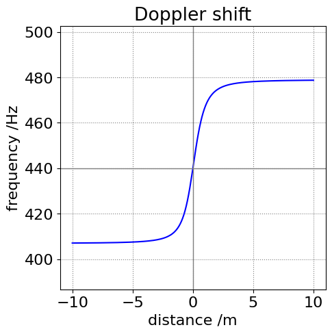
Figure 32. The relative apparent change in the siren’s frequency as an ambulance passes when approaching from the right and when 1 m away from the kerb. Notice that the curve is not symmetrical about 440 Hz.
(b) Rearranging the frequency equation into two parts,then dividing top and bottom by \(s\), produces
Expanding in terms of \(v/v_s\), as this is a small speed (\(60/740\)) gives
As \(v_0\), the speed of the observer is also very small compared to the speed of sound this makes \(v_0/v_s \to 0\) and the fractional change in frequency approximately
The squared term can be ignored because \(v\lt s\) and finally, therefore
Using the values given in the question, the perceived frequency is \(1.08f_0\) and the change is \(f_0 \cdot 60/740 = 0.08 f_0\). If the siren works at \(440\) Hz, A on a musical scale, the change in frequency is only \(32.5\) Hz or by \(1.074\) times. This ratio is a change in frequency by slightly more than a minor second which would be an increase of \(2^{1/12} = 1.059\) times, but less than a major second, which would be an increase of \(2^{2/12} = 1.122\) times.
In our example, the perceived frequency is constant at \(1.08f_0\) as the ambulance approaches us, but because we are, hopefully, on the roadside and not in the middle of the road, our angle to the vehicle changes as it is moving. Consequently, we hear the frequency decrease in proportion to the apparent velocity of the vehicle and the angle between the direction of travel and ourselves. This means that the frequency decreases imperceptibly slowly when the vehicle is a long way off but more rapidly as it approaches. It is exactly \(f_0\) just at the instant it passes, and then falls further as it recedes to a final value of \(0.92f_0\). Different vehicle and sound speeds and your position will of course, give different perceived frequencies.
Q39 answer#
(a If the star is moving slowly relative to us then \(v/c \ll 1\) and letting \(v/c = x\) then expanding the square roots as \((1 + x)^{1/2}(1 - x)^{-1/2}\), which avoids dividing the expansions produces,
Multiplying and keeping only constants and terms in \(x\) and \(x^2\) produces \((1 + x)^{1/2}(1 - x)^{-1/2} = 1 + x + x^2 \cdots\) and as \(x = v/c\) substituting into the equation in the question gives \(\delta \lambda /\lambda = v/c \) to first order.
(c) As the reference transition is 0.1 nm wide then using the wavelength for the Lyman-\(\alpha\) line \(4 \cdot 10^7/3R = 121.5\) nm, the star velocity is \(v = 3R\Delta \lambda c/(4 \cdot 10^7\)) and the minimum velocity is half this because of the resolution limit and is \(\approx 1.23 \cdot 10^5\,\mathrm{ m\, s^{-1}}\); very approximately four thousandths of the speed of light.
Q40 answer#
(a) When \(V\) = 0 the levels must be \(E_1\) and \(E_2\) as nothing has perturbed them. With the perturbation present \(V \ne 0\) and the total energy is, with \(\Delta E = E_2 - E_1\),
which is unchanged.
(b) When the coupling \(V\) is small the square root can be expanded in \((V/\Delta E)^2\). Rewriting the equation as
and then expanding produces
from which
This approximation is good at small coupling \(V\) as seen in the figure below. When \(V \gg \Delta E\) using equation 30 produces \(\displaystyle E_\pm =\frac{E_1}{2}+\frac{E_2}{2}\pm V\) and this is the large energy limit approximation shown by the straight lines in the figure below. This limit is inaccurate at small coupling \(V\) as might be expected.
fig1= plt.figure( figsize=(5, 5) )
E2 = 4
E1 = 2
deltaE= E2 - E1

fEp = lambda V: (E2 + E1 + np.sqrt(deltaE**2 + 4*V**2))/2.0   # exact
fEm = lambda V: (E2 + E1 - np.sqrt(deltaE**2 + 4*V**2))/2.0

numx= 100
x  = np.linspace(0,3,numx)

Ep =[fEp(x[i]) for i in range(numx)]                # exact
Em =[fEm(x[i]) for i in range(numx)]

Elimp = [ (E1+E2)/2.0+x[i] for i in range(numx)]     # limiting value x represents V
Elimm = [ (E1+E2)/2.0-x[i] for i in range(numx)]

Eaprxp= [E2 + x[i]**2/deltaE for i in range(numx)]  # approximation
Eaprxm= [E1 - x[i]**2/deltaE for i in range(numx)]

plt.plot(x,Ep,color='black',linestyle='solid',label='exact E+')
plt.plot(x,Em,color='black',linestyle ='solid')

plt.plot(x,Elimp,color='blue',linestyle='dashed',linewidth=1,label='limit '+ r'$V/\Delta E > 1$')
plt.plot(x,Elimm,color='blue',linestyle='dashed',linewidth=1)

plt.plot(x,Eaprxp,color='red',linestyle='dotted',label='approx '+ r'$\Delta E/V < 1$')
plt.plot(x,Eaprxm,color='red',linestyle='dotted')

plt.ylabel('Energy')
plt.xlabel('V')
plt.axis([0,3,-4,10])
plt.legend(fontsize=12)
plt.show()
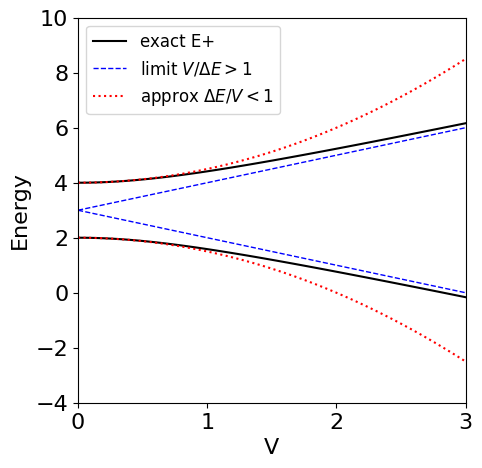
Figure 33. Exact energies (dashes), equation (30), and curves in the limit when the ratio \(V/\Delta E\) is small (solid) and large (dotted) vs coupling energy \(V\).
The interaction energy \(V\) is often a fixed quantity in a molecule as it depends upon the shape of the potential energy surface. However, \(V\) can be made to change if, for example, an electric or magnetic field is present. The former leads to the Stark effect, the latter would represent the Zeeman effect. The Nuclear Zeeman effect, which alters the energy of nuclear spin states, leads to NMR spectroscopy.
Q41 answer#
Suppose that the ions are alternately charged, \(q=\pm eZ\) and the energy is the sum of all the terms. As each ion has an equal but opposite charge, the charge number can be taken out of any calculation and the result multiplied by \(Z\). The smallest separation between two charges is \(d\), the next \(2d\), then \(3d\) and so on. Therefore, choosing a victim positively charged ion, shown in the top part of Fig.9, its Coulomb energy is the sum of that due to pairs of ions at separation \(d\), \(2d\), \(3d\) ignoring the ions in between any particular pair. It does not matter which ion you start with because the chain is infinitely long. If it were of a fixed length, it still would not matter as long as each interaction is only counted once.
The total energy of half of our infinite chain is the series
and, obviously, the sign of each terms alternates because the ions are alternatively positive and negative. This is half the energy because ions were counted only to the right of our victim. The series can be simplified and terms collected to form
The next step is to look at a table of expansions to see if the terms in square brackets form a known series. Doing this gives \(\ln(1+x)=x-x^2/2 +x^3/3 -\cdots \) and when \(x\)=1 produces \(\ln(2)=1-1/2+1/3-1/4 -\cdots\) which will do very nicely. The total energy is therefore
where the result is multiplied by \(2\) to account also for the ions to the left of our victim ion. The Madelung constant for the linear chain is therefore \(2\ln(2) = 1.386\).
The summation of terms in the square bracket can be checked numerically. The terms to sum are \((-1)^{j+1}/j\)
s = sum( (-1)**(j+1)/j for j in range(1,1000) )
print(s)
0.6936474305598223
Adding more terms to the summation makes the result closer to the correct answer, but convergence is terribly slow. (b) The calculation with the square lattice is a little more complex. Using Pythagoras, the distance of an ion \(md\) and \(nd\) units away from our victim ion at the origin is that of the hypotenuse of a triangle of side of \(m\) and \(n\) units of length \(d\), which is \(d\sqrt{m^2 + n^2}\) ; therefore the contribution to the energy is \(\displaystyle \frac{q}{d\sqrt{m^2+n^2}}\) for an ion of charge \(q\). The constant \(d\) is the length of the side of the grid and can be taken outside any summation.
The calculation becomes one to add together; \(n\) rows each of \(m\) ions with \(m\) and \(n\) varying from \(\pm \infty\), but remembering to change the sign from \(-1\) to \(+1\) to take into account the change in charge of the ions. Infinity in this calculation means use a large enough number of rows and columns to make the summation converge; let ‘infinity’ be the number \(s\). Referring to the diagram for the row with \(n = 1\), the lattice terms are
as \(m = 0, 1, 2, 3 \cdots\). This summation can be represented as
The second row with \(n = 2\) produces
which has the summation
The total energy is therefore given by
The sum is over all \(n\) and \(m\) points in the lattice starting line, from an ion at position \(-s\) to one at \(+s\), is the double summation,
which was obtained by induction. The instance when \(m = n\) = 0 has to be excluded because this represents the distance from the origin to the origin. This does not make physical sense, as it is zero and would lead to infinity in the sum. If there are \(s\) indices, the summation must extend from \(m = -s \cdots +s\) and similarly for \(n\) to add in ions with negative indices; see Fig. 9.
In the numerical summation because of the reciprocal distance dependence of each energy term and the alternating charges, the terms converge very, very slowly and each summation needs at least \(200\) terms, which if made bigger may take some time to calculate.
# 2D Madelung constant , square lattice.

f01 = lambda m,n :((-1)**(m+n))/np.sqrt(m**2 + n**2) if (m**2 + n**2) != 0 else 0.0
                                            # m^2=n^2 to stop +-n+-m=0
s = 200
aterms = [[ f01(n,m) for n in range(-s,s+1)]  for m in range(-s,s+1)  ]
                                            # s+1 to make indices go from -s ..0..s
M = sum( map( sum, aterms) )
print(M)
-1.6120159150827391
# conventional type of code makes the calculation slightly faster.
sm = 0.0
for n in range(-s,s+1,1):
    for m in range(-s,s+1,1):
        temp = n**2 + m**2
        if temp != 0:
            sm = sm + (-1)**(n+m)/np.sqrt(temp)
print(sm)
-1.6120159150827853
With 200 terms the result is \(-1.612\), this Madelung constant makes the energy
The three-dimensional version can be realized by extending this calculation, but convergence is so slow that it will take an inordinately long time to calculate an accurate result. In practice, different formulae are needed for accurate summation in this calculation because the series converges so slowly that rounding errors, caused by adding and subtracting similar valued numbers, may accumulate giving incorrect answers.
Q42 answer#
Using the figure there are six face-centred atoms of type A, twelve edge-centred of type B and eight corner atoms of type C. The summation of these atoms is
More distant atoms in the next unit cells are \(24\) type A′ at \(R\sqrt{5},\, 24\) type B′ at \(R\sqrt{6},\, 24\) corner atoms at \(R\sqrt{11},\, 6\) atoms with \(R2\sqrt{6}\), projected though atoms C and so on.
Very soon, it becomes very hard to count them all and furthermore it may be necessary to go to further cubes if the summation does not converge. Using python the summation is far easier than by hand. The atoms can be defined at integer values on a grid, \(000, 111, 101\), and so forth with minimum atom separation \(R\), then all the distances are easily calculated by Pythagoras’ theorem in units of \(R\). This can then be given a length of one to further simplify the calculation.
# 3D cubic lattice Lennard-Jones  6-12 energy
#----------------------
def fn(n,i,j,k ):                    # calcuate distances , return 1/alpha^n or zero.
    a = np.sqrt(i**2 + j**2 + k**2)
    if a != 0:
        return 1.0/a**n
    else:
        return 0.0
#----------------------
s = 5                    # size of lattice i,j,k
for p in [6,12]:         # calculate for both alpha^ 6 and 12
    M = [[[ fn(p,i,j,k) for i in range(-s,s+1,1)] for j in range(-s,s+1,1)] for k in range(-s,s+1,1)]  # 3D list
    total = np.sum( M )  # sum all values in 3D list
    print('{:s}{:s}{:s}{:f}'.format('1/alpha^',str(p),' = ',total))
    pass
1/alpha^6 = 8.387116
1/alpha^12 = 6.202149
The \(\alpha^6\) sum converges much more slowly than that for \(\alpha^{12}\) and the value found is only accurate to a few decimal places.
Exercise: Calculate the lattice sums for body centred and face centred cubes by adding or removing selected lattice points.
Q43 answer#
Expanding the dipole \(\mu\) as a Taylor series in the extension \(x\) produces
where \(\mu_0\) is the dipole at the equilibrium extension \(x = 0\), i.e. when the bond displacement is zero. Note the units; the dipole \(\mu\) and \(\mu_0\) is measured in Debye which are coulomb metres, the first derivative has units of charge, i.e. coulomb, the second C/m, and so forth.
(a) The harmonic oscillator has a dipole that is linearly proportional to extension so that \(d\mu/dx|_0 \) is a constant and thus higher derivatives are zero. Of course, \(d\mu/dx|_0\) must itself not be zero which it is in homo-nuclear diatomic molecules, and therefore these molecules do not have a vibrational absorption spectrum.
Experiment tells us that the dipole in HCl is \(1.085\) Debye(D) and \(d\mu/dx|_0\) is about \(0.86\cdot 10^{-8}\) C. (\(1 \mathrm{D} = 3.33 \cdot 10^{-30}\) C m).
By substituting for \(\mu\) the transition moment integral becomes
As the wavefunctions in any given state are orthogonal to one another and the initial state \(i\) clearly cannot also be the final state \(f\), therefore \(\displaystyle \int \psi_j^*\psi_i dx=0\) The transition moment is simplified to
The integral is not zero if the vibrational quantum number of state \(f\) is \(f = i + 1\), because of the odd-even character of the vibrational wavefunctions, which are the Hermite polynomials, see question Q50.
(b) The anharmonic oscillator has a dipole that varies in some non-linear way with extension, therefore additionally \(d\mu/dx|_0 \ne 0\) are present in the transition moment integral that becomes,
in which the second integral is zero if \(f=\pm i+2\). In practice \(d^2\mu/dx^2|_0\) is small and the transitions with \(\Delta \nu -f-i =\pm 2\) are only weakly observed and are called the first overtone or second harmonic transitions.
Q44 answer#
(a) In this particular example \(\displaystyle \frac{dU}{dE}= \left<\frac{dH}{dE} \right>\), therefore, the derivative is easily calculated and is from the equations in the question, \(\displaystyle dU/dE = -\langle \mu_z \rangle \).
(b) Expanding the energy as a Taylor series in electric field \(E\), by definition,
where subscript 0 implies that the derivatives are calculated when \(E = 0\) and \(U_0\) is the molecular energy at zero field.
(c) From part (a), \(\langle \mu_z \rangle \) can be written down as the derivative of \(U\), therefore
and comparing this equation with the definition in the question \(\displaystyle \langle \mu_z \rangle =\mu_{z0}+\alpha E+\beta E^2/2\) the following identifications can be made,
and therefore the energy is