
5 Appendix: Some basic Python instructions with a few examples.
Contents
5 Appendix: Some basic Python instructions with a few examples.#
# First import all python add-ons etc that will be needed later on
# the next line is specific 'magic' instruction to jupyter notebook ; do not add anything ele to that line
%matplotlib inline

import numpy as np               # general python    fast numerical calculation
import matplotlib.pyplot as plt  # general python    plotting  always used

from scipy.integrate import quad # specific use: e.g. import general numerical integration routine;

from sympy import *              # algebraic solution of equations, only add if doing algebraic things
init_printing()                  # allows printing of SymPy results in typeset maths format
plt.rcParams.update({'font.size': 14})  # set font size for plots, alter at will.
5.1 Basic syntax. Python 3 is assumed.#
(1) The position an instruction starts on a line is important. Normally position zero starts a line but in loops or after conditional statements indented by 4 spaces or a tab. In general it seems that the spaces and tabs cannot be mixed.
(2) Python is case sensitive, i.e. a name \(\mathtt{Func}\) is different to \(\mathtt{func}\). Names should not start with a number.
(3) \(\sqrt{-1}\) is given the symbol \(\mathtt{1j}\) or \(\mathtt{1J}\)
(4) Division takes two forms, a/b for normal floating point, i.e. 3/2 = 1.5 and a//b for integer division, i.e. 3//2 = 1
(5) Functions sin, cos or your own function use round brackets i.e. \(\mathtt{np.tan(x)}\), where \(x\) can be floating point or integer and the function is evaluated at hat value.
(6) Arrays/lists use square brackets, e.g. \(\mathtt{myary[i]}\) and integer index, \(i\), and returns the value at that index.
(7) Normal functions sin, cos etc. are unknown and have to be accessed via NumPy as \(\mathtt{np.sin(x), \;np.exp(x),\; np.pi }\) etc. Use NumPy for any numerical calculation other than trivial ones as it is fast.
(8) Powers are made as \(\mathtt{x**(1J+3)}\) etc.
(9) Indexing lists, sets, and arrays all start at zero, i.e. the first element of mylist is, \(\mathtt{mylist[ 0 ]}\). If the list is of length \(n\) the last element is \(\mathtt{mylist[n-1]}\)
(10) When using for loops, while loops, subroutines, if statements, etc. the first line ends in a colon: for example
f01 = [ i**2 for i in range(10) ]   # define list
for i in range(10):                 # this has values ten values, i from  0 to 9  end in :
    f01[i] = i*10.5
print(f01[:])                       # the colon means use whole list
[0.0, 10.5, 21.0, 31.5, 42.0, 52.5, 63.0, 73.5, 84.0, 94.5]
and all lines in the loop are inset by 4 spaces or a tab.
(11) Loops, subroutines, if etc. have no end statements; the tabbing is enough to delimit the range, however, it is acceptable to add the word pass as the last statement as it often makes reading easier.
(12) There are objects called list comprehensions that are an alternative to loops in many cases. They are more concise but for speed or complex cases use loops.
mylist = [ i+2 for i in range(6) ]    # makes list of 6 values, i = 0 to 5 see below for details
mylist[:]

Arrays are usually called lists and enclosed by square brackets \([\; ]\) and indexed by square brackets, e.g. \(\mathtt{mylist=[ 2, 3, 4 ]}\) and so to print use
print( mylist[ 0 ] )
2
to print the first element.
(13) In Python 3 notice that print statements are always enclosed in round brackets. To print the whole list use,
print(mylist)             # or
print(mylist[ : ])
[2, 3, 4, 5, 6, 7]
[2, 3, 4, 5, 6, 7]
(14) Printing using f’’ notation
A new and quick method to print is using f notation, thus to print ‘ one fifth = 1/6 ‘ we could use
print('one sixth =', 1/6)  # or formatted as
print('{:s}{:6.3f}'.format('one sixth =', 1/6))
one sixth = 0.16666666666666666
one sixth = 0.167
we can use the f format but note that only the last occurrence of this is printed in any cell
f'one sixth = {1/6:6.3f}' # the .3 gives 3 decimal places, the 6 is ignored but can be included
'one sixth = 0.167'
(15) 2D lists are called as \(\mathtt{A[ i ][ j ]}\) , i.e. two separate brackets.
NumPy arrays are called in a similar manner however, 2D arrays can be called differently as \(\mathtt{A[ i, j ]}\) with one square bracket.
(16) To convert an array to a NumPy array use \(\mathtt{ np.array([2,3,4]) }\)
5.2 Functions#
There are two types of user defined functions, as in a multi-line subroutine or procedure e.g.
def myfunc(x):           # use this for complicated function with if else etc
    return x*np.sin(x)
print(myfunc(np.pi/3))
0.9068996821171088
and in a lambda or single line statement, e.g.
myfunc = lambda x : x*np.sin(x)     # use for one line functions

print(myfunc(np.pi/3) )
0.9068996821171088
5.3 Importing packages#
It is necessary to import other packages for specific calculations, NumPy for fast numerical calculations, SciPy for special functions (such as error function), integrations, non-linear least squares etc. and matplotlib for plotting. SymPy is used for algebraic calculations.
5.4 Integer division#
The other main different to earlier python than version 3 is that 3/2 is treated as real division,i.e. 1.5. To get integer division use 3//2 = 1. This is important if the division is then to be used as an index as these can only be integers.
5.5 Simple statements, printing formats#
a = 2.1**3.1               # raise to power
b = np.sin(2*np.pi*a)      # use numpy to define sine and pi
c = 123
print(a,b,c)               #  quick print
print('{:s}{:6.3f}{:s}{:6.5g}{:s}{:4d}'.format('The value of a is ', a , '\nThe value of b is ',b, ', c is ',c))

# print uses s for string, f for reals, d for integer, g for general real, e  for scientific if needed
# \n causes a newline
9.97423999265871 -0.1611491390171008 123
The value of a is  9.974
The value of b is -0.16115, c is  123
6 Lists and List comprehension#
Often a list (called an array in other languages) has n values that can be addressed later on. In python these can be number or strings of letters etc. or a mixture of these. Strings are enclosed in parenthesis as ‘a’.
Usually a name is chosen and then values added in a loop of some kind. In many cases in python this can be done in one go. This is called list comprehension, see how a is generated below. Also shown is how different values can be extracted. The statement \(\mathtt{range(5)}\) in the code below has values 0 to 4 because the first value in the list has zero index so is given by a[0].
# printing and intro to list comprehension

a = [np.sin(i*np.pi/4) for i in range(5)]  # list comprehension, range makes list of 5 values where i varies from 0 to 4
                                           # this is alternative to a 'for' loop
print('list is ', a)

print('4th value is a[3] = ', a[3])                  # print 4th value as index starts at zero
print('1st to 3rd value is a[0:3] = ', a[0:3])
print('last value a[-1] =',a[-1])
print('reverse order a[::-1] =', a[::-1])            # note double ::
list is  [0.0, 0.7071067811865475, 1.0, 0.7071067811865476, 1.2246467991473532e-16]
4th value is a[3] =  0.7071067811865476
1st to 3rd value is a[0:3] =  [0.0, 0.7071067811865475, 1.0]
last value a[-1] = 1.2246467991473532e-16
reverse order a[::-1] = [1.2246467991473532e-16, 0.7071067811865476, 1.0, 0.7071067811865475, 0.0]
print('The values in my list are as follows')
for p in a:                                  # note colon and we call whole list
    print('{:6.3f}'.format(p))               # format a list, note indent

print('Second method; use enumerate to get index and values')
for i, p in enumerate(a):
    print('{:4d} {:6.3f}'.format(i,a[i]))

print('Third method; print directly as in conventional programming loop to get index and values')
for i in range(5):                                   # call individual values
    print('{:4d} {:6.3f}'.format(i,a[i]))            # format a list

print('Fourth method part of list')                  # use list to define spcific values
for i in [0,3,4]:
    print('{:4d} {:6.3f}'.format(i,a[i]))
The values in my list are as follows
 0.000
 0.707
 1.000
 0.707
 0.000
Second method; use enumerate to get index and values
   0  0.000
   1  0.707
   2  1.000
   3  0.707
   4  0.000
Third method; print directly as in conventional programming loop to get index and values
   0  0.000
   1  0.707
   2  1.000
   3  0.707
   4  0.000
Fourth method part of list
   0  0.000
   3  0.707
   4  0.000
6.1 Use list comprehension to make a double list#
Rather than use a double loop to put values into a double list this can be done in one go as follows.
b = [ [ np.exp(-i*j) for i in range(5)] for j in range(3) ]  # 2d list, b[j][i] ,i.e. 2nd index in first place

print('\ndouble list is')
print(b)
print('\ndouble list index in order b[j][i], second row, fourth column has value b[1][4]', b[1][4] )
print('printing b[4][1] will lead to an error e.g.')
#print(b[4][1])       the error produced here will stop the notebook code cell from continuing until it is fixed.
double list is
[[1.0, 1.0, 1.0, 1.0, 1.0], [1.0, 0.36787944117144233, 0.1353352832366127, 0.049787068367863944, 0.01831563888873418], [1.0, 0.1353352832366127, 0.01831563888873418, 0.0024787521766663585, 0.00033546262790251185]]

double list index in order b[j][i], second row, fourth column has value b[1][4] 0.01831563888873418
printing b[4][1] will lead to an error e.g.
7 Numerics are much faster with NumPy.#
Import NumPy (see top of page) to use mathematical functions and make arrays. The operation is orders of times faster than basic Python.
x = np.linspace(0,10*np.pi,5)  # make x range from 0 to 10pi in 5 steps.

myary = np.zeros((5,3),dtype=float)  # 2D array of size 5 by 3 (row, col)  full of zeros

for i in range(5):
    for j in range(3):
        myary[i,j]= np.sin(x[i])*np.exp(-j/10)
print(myary[:,2])        # print all of column 2 which is 3rd as index starts at 0
myary[:,:]
[ 0.00000000e+00  8.18730753e-01  5.01327998e-16 -8.18730753e-01
 -1.00265600e-15]
array([[ 0.00000000e+00,  0.00000000e+00,  0.00000000e+00],
       [ 1.00000000e+00,  9.04837418e-01,  8.18730753e-01],
       [ 6.12323400e-16,  5.54053124e-16,  5.01327998e-16],
       [-1.00000000e+00, -9.04837418e-01, -8.18730753e-01],
       [-1.22464680e-15, -1.10810625e-15, -1.00265600e-15]])
8 Append to a list#
Appending one value at a time to a list is a very useful way of lengthening a list when the final length is unknown. Can be useful when reading datafile whose length is unknown. Start with an empty list then use a loop.
mylist = []                    # empty list
lim_value = 3                  # e.g. some value determined by programme else where

i = 0
while i <= lim_value:
    if i != 1:
        mylist.append( np.exp(-i**2/3))  # add value to list
    i = i + 1                  # you must increment index in a while loop
print(mylist)
[1.0, 0.26359713811572677, 0.049787068367863944]
8.1 Using loops and if else to calculate stuff. How to make sum of terms#
f01 = [ 0.0 for i in range(20)]         # make list full of zeros

for i in range(20):                     # range i from 0 to 19
    if i != 0 :                         # use if not equal to zero
        f01[i] = np.sin(2*np.pi/i)**2
    else:
        f01[i] = 1.0
    pass

print(f01)                               # print whole list

print('\nsum of whole list is ', sum(f01) )  # use just for 1D list, use numpy sum for anything else
[1.0, 5.99903913064743e-32, 1.4997597826618576e-32, 0.7500000000000003, 1.0, 0.9045084971874736, 0.7499999999999999, 0.6112604669781571, 0.4999999999999999, 0.41317591116653474, 0.3454915028125263, 0.2922924934990568, 0.24999999999999994, 0.21596762663442207, 0.18825509907063323, 0.16543469682057085, 0.14644660940672624, 0.13049554138967043, 0.11697777844051097, 0.10542974530180318]

sum of whole list is  7.885735968708085
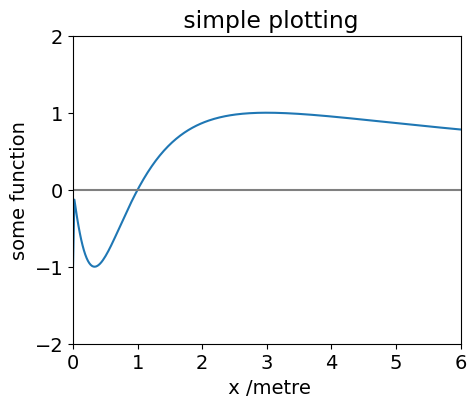
Now do same calulation but instead of using i to determine values in the sine function we define x and give it values then we will plot the result. (If you want to alter the size of the plot then figure has to be used, see drawing two plots, somewhere below this cell).
numx = 300                              # number of points
f01  = [ 0.0 for i in range(numx)]      # make list full of zeros
# you could also use NumPy to do this
# f01 = np.zeros(n,type=float)

x = np.linspace(0,2*np.pi,numx)         # make numx values evenly spaces between 0 and 2pi

for i in range(numx):                   # range sets values, in this case x and f01 must have same length
    if x[i] != 0 :                      # use if not equal to zero
        f01[i] = np.sin(2*np.pi/(x[i]+1))       # fill list elements with values
    else:
        f01[i] = -1.0
    pass

#print(f01)    # printing disabled as 300 points
figx = plt.figure(figsize=(5, 4))
plt.plot(x,f01)                       # must have imported matplotlib, this is done at top of worksheet
plt.xlim([ 0, 6 ])
plt.ylim([ -2, 2])
plt.xlabel(' x /metre')
plt.ylabel( 'some function')
plt.title( ' simple plotting')
plt.axhline(0,color='grey')
plt.show()                            # this must be last plotting instruction
If you want to plot two graphs together then it is a bit more complicated. First it is necessary to define a figure and then define axes on which to draw the data and add subplots as the two figures. This is shown below.
9 Functions.#
There are standard functions sin, cos, exp etc. that we use NumPy to call as np.sin(x) etc. There are also two main types of user defined function that can take arguments.
9.1 Lambda functions; more examples#
These are very useful single line functions. They have the form
aname = lambda variable1, variable 2, etc. : expression in variables 1, 2 etc.
note the word lambda and the colon.
These function are called using normal parentheses, i.e. curved brackets as \(\text{aname(3.0,2.0,...)}\) Note that in contrast, lists use square brackets.
It is also possible to use if statements inside a lambda and an example is given but it is usually better to use a def type function.
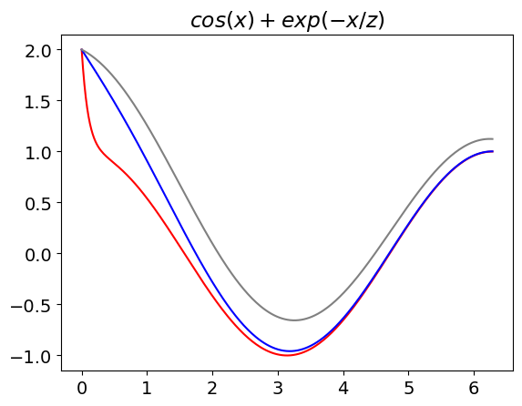
func1 = lambda x, z : np.cos(x) + np.exp(-x/z)        # define function in x and z

print( func1(3.1,4.2) )                               # print value at given x and z

func2 = lambda x, z: np.sin(x) if z <= 0 else  np.cos(x) + exp(-x/z)  # you can do this but its better to use def type functions

print('func2 with if statement, cannot plot this, value at -1 is ', func2(1.0,-1) )

x = np.linspace(0,2*np.pi,300)      # define x values

plt.plot(x, func1(x,0.1),color='red' )    # example of plotting lambda function, note how x is whole list of values
plt.plot(x, func1(x,1.0),color='blue')
plt.plot(x, func1(x,3.0),color='gray' )
plt.title(r'$cos(x)+exp(-x/z)$')           # plot using mathjax , put r before ' bla bla' and enclose in $ signs
plt.show()
-0.5211115802791633
func2 with if statement, cannot plot this, value at -1 is  0.8414709848078965
9.2 def functions#
These are the more general type of user defined functions and allow for any sort of complicated function. They are the equivalent of subroutines in other languages.
The answers you want are obtained by using a return statement.
The variables inside the function are local, i.e. if you use x inside its different to the x outside. However, there are rules on local and global variables that need checking.
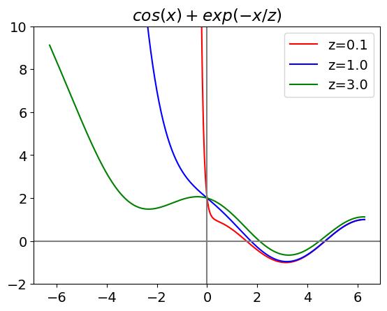
The syntax for def functions is shown below. Note also that we can now plot negative values of our function, not possible with the way the lambda function was defined.
def afunc(x,z):                              # define afunc to be function of x and z

    if z <= 0:                               # can add if else and loops etc. inside def function.
        ans = np.sin(x)
    else:
        ans = np.cos(x) + np.exp(-x/z)
    return ans, 2*x, np.sin(z)               # must use return (and as many values as you want )

Q, is_x, is_z = afunc(3.1,4.2)               # return sends three values back, call them Q, is_x, is_z

print('returned values are Q, 2*x and sin(z), i.e.',Q, is_x, is_z)

x = np.linspace(-2.0*np.pi,2*np.pi,300)      # define x values with numpy:  (start, end, num points)

col=['red','blue','green']                   # choose colours then index in loop

for j, z in enumerate([0.1,1.0,3.0]):         # enumerate passes  index , value  into loop
    plt.plot(x, func1(x,z),color = col[j], label='z=' + str(z) )    # example of plotting lambda function, note how x is whole list of values
    pass

plt.ylim([-2,10])
plt.title(r'$cos(x)+exp(-x/z)$')             # plot using mathjax , put r before ' bla bla' and enclose in $ signs
plt.axhline(0,color='gray')
plt.axvline(0,color='gray')
plt.legend()
plt.show()
returned values are Q, 2*x and sin(z), i.e. -0.5211115802791633 6.2 -0.8715757724135881
9.3 Recursive functions#
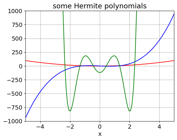
It is possible to make functions recursive, calculating a factorial as \(n! = n.(n-1).(n-2)\cdots 1\) is the commonly used example and is given below as is one to calculate Hermite polynomials used in determining harmonic oscillator wavefunctions.
def fact(n):                    # factorial cannot be used for huge values
    if n == 0 or n == 1:
        return 1
    else:
        return n*fact(n-1)      # call the function again until we get 1, jump out and end with return 1
#-------------------------

print('number factorial')
for i in range(10):
    print ('  ', i, '     ',fact(i))
number factorial
   0       1
   1       1
   2       2
   3       6
   4       24
   5       120
   6       720
   7       5040
   8       40320
   9       362880
def Hermite(n,x):   # use recursion formula, x is real, n is order. H(n,x) = 2.x.H(n-1,x)-2.(n-1).H(n-2,x)
    if n == 0:
        return 1
    elif n == 1:
        return 2*x
    else:
        return 2*x*Hermite(n-1,x) - 2*(n-1)*Hermite(n-2,x)
#--------------

x = np.linspace(-5,5,100)                       # define x range with 100 points
plt.plot(x, Hermite(2,x),color='red')
plt.plot(x, Hermite(3,x),color='blue')
plt.plot(x, Hermite(6,x),color='green')
plt.axis([-5,5,-1000,1000])
plt.xlabel('x')
plt.title('some Hermite polynomials')
plt.grid()
plt.show()
10 Using map( f(x), alist ) or [ f(x) for x in list ]#
This is a way to perform an operation of a list of things without having to use a loop. The map function has two or more arguments map( function, sequence ). One simple use is to multiply all of a list by some number, you cannot do *[1,2,4,5]2 for example, but have to use map or list comprehension as shown below.
# using map
alist = [1,2,4,5,7,9]
blist = list( map( lambda x: x**2, alist) )  # square list;  note have to add list() to get result.
print('blist',blist)

# using list comprehension:  does not matter which is used. This method seems clearer to me though
clist = [x**2 for x in alist]
print('clist',clist)

dlist= list(map(lambda x ,y: x**2 + y , alist, blist))  # square alist then add to blist.
print('\ndlist',dlist)

elist = list( map(np.sin, dlist) )                       # make sine of each term
print('\nelist', elist)

eelist = [ np.sin(x) for x in dlist]                    # alternative
print('eelist', eelist)

# make characters from a ascii numbers

numlist = [ 72, 65, 84 , 82, 88, 32 ,73 ,83 , 32, 66 ,69 , 83, 84 ]
alpha = list( map( chr, numlist) )
print('\n',alpha)
print("\nremove ' and , from output", str(alpha).replace("'",'').replace(',',''))  # remove ' and ,
blist [1, 4, 16, 25, 49, 81]
clist [1, 4, 16, 25, 49, 81]

dlist [2, 8, 32, 50, 98, 162]

elist [0.9092974268256817, 0.9893582466233818, 0.5514266812416906, -0.26237485370392877, -0.5733818719904229, -0.9784503507933796]
eelist [0.9092974268256817, 0.9893582466233818, 0.5514266812416906, -0.26237485370392877, -0.5733818719904229, -0.9784503507933796]

 ['H', 'A', 'T', 'R', 'X', ' ', 'I', 'S', ' ', 'B', 'E', 'S', 'T']

remove ' and , from output [H A T R X   I S   B E S T]
11 Algebraic and numerical integration of a function#
Now we will do some integration, both algebraic and numerically; we have already imported integrate from SciPy; see top of document.
The function to integrate is first defined and plotted.
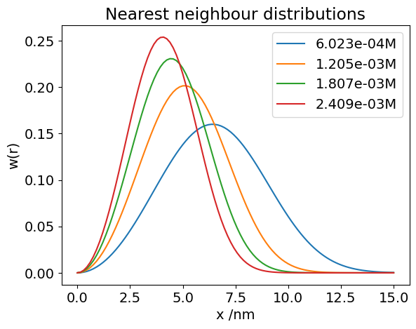
The calculation of nearest neighbour distances from one molecule to another has been worked out see Chandrashkar, Rev Mod Phys 1943.
Let \(w(r)\) be the probability that the nearest neighbour occurs between distance r and r+dr. This must be the probability than no molecules exist closer to the victim molecule that one occurs at a distance r and that this molecule exists in the shell r to r+dr. Thus,
where n is the average number of molecules / unit volume. (1 mol \(\equiv 10^3N_A/10^{27} = 0.6023 \) molecules / nm\(^3\)).
This is hard to solve as it is because \(w(r)\) is also inside the integration, so it is necessary to differentiate to find a result which is;
# plotting the distribution for some concentrations. Use n in molecs/nm^3, r in nm

w = lambda r,n : 4*np.pi*r**2*n*np.exp(-4*np.pi*r**3*n/3.0)   # define function w(r) with variables r and n

maxr = 15.0       # max distance in nm
numr = 100        # number of data popints
n0   = 0.6023     # number molecs/nm^3 at 1 mole

r = np.linspace(0, maxr, numr)         # make list of distances

for i in range(1,5):                   # note :  range 1 to 4
    n = n0*1e-3*i                      # 1e-3 to make millimolar; convert to number/nm^3
    plt.plot( r, w(r,n), label = str('{:4.1e}'.format(i*1e-3)) + 'M')   # can put print format into string

plt.ylabel('w(r)')
plt.xlabel('x /nm')
plt.title('Nearest neighbour distributions')
plt.legend()
plt.xlim([0,15])
plt.show()
12.1 Symbolic algebraic integration; example to find average distance#
The average distance given the distribution \(w(r)\) is \(\displaystyle \langle r \rangle = \int_0^\infty rw(r)dr\). The integral can be performed in the normal way but we use SymPy to illustrate this. The steps are to define symbolic constants then do the integration.
In SymPy infinity is oo (two lower case letter o). The conds=’none’ removes any periodic conditions and so simplified the result.
# average distance algebraically using SymPy
n,r = symbols(' n, r')                       # define symbols to use SymPy . Note also that pi and exp are known by SymPy.

f01 = 4*pi*r**3*n*exp(-4*pi*r**3*n/3)       # note that we do not use np.exp or np.pi as SymPy knows functions
av=  integrate(f01,(r,0,oo), conds = 'none')  # use conds ='none' if you are happy that no funny results are expected.
av

The result contains the gamma function, if you type \(\mathtt{av.evalf()}\) you can evaluate the numerical parts and find that \(\displaystyle \langle r \rangle = 0.55396n^{-1/3}\), which is \(6.56\) nm at \(10^{-3}\) M.
12.2 Numerical integration#
The same calculation can be done numerically of course, but in that case n has to be defined in each instance.
# using SciPy numerical integration  quad(func, x_start, x_end, arg( arguments in user function other than x))
# the quad() returns two values the integration and the error bound.
# the user define function below if called func (we are so imaginative)
# but could also de defined as _def myfunc(r,n):_ etc.
# general purpose integration.
# Must have loaded scipy integration here if not done above.
# it is always necessary to plot function first otherwise integration range may be unkonwn
# and integration may still converge properly but the result be in error.

func = lambda r, n : 4*np.pi*r**3*n*np.exp(-4*np.pi*r**3*n/3.0)     # user define function to integrate,

                            # r is variable  to integrate over, this need not be defined as quad() defines this.
n = 1e-3*0.6023             # number molecules 1 mol/dm^3 equals this number at  1 mol /nm^3
maxr = 30.0                 # integration range
minr = 0.0

av, err = quad(func, minr, maxr, args=(n))
                             # in args only put variable name(s) from function not integrated over.
                             # err is error bound, you should check this for convergence

if err < 1e-6:
    print('{:s}{:f}{:s}{:f}{:s}{:f}'.format('molecs/nm^3 = ',n,' numerical = ', av, ' exact = ', 0.55396/n**(1.0/3.0)))
else:
    print('{:s}{:g}'.format('error too large ',err))
molecs/nm^3 = 0.000602 numerical = 6.559554 exact = 6.559551
13 Some other algebraic calculations, differentiation and series#
SymPy can be used in the same way as Maple or Mathematica to perform algebra. It is quite easy but the manuals are complicated and so a couple of examples are given below.
First differentiating then generating series expansion of the function produced. The first step is to define the symbols to be used. We will use the nearest neighbour distribution to begin with. The best output results are found without using print() as shown below. If you do use print as in print(Q.doit() ) a code type output is produced and the nice output suppressed.
# assume SymPy already loaded.

n,r = symbols('n, r')                       # define symbols to use .
                                            # Note also that pi and exp are known by SymPy.

f01 = 4*pi*r**3*n*exp(-4*pi*r**3*n/3)

Q = simplify( diff(f01,r) )                 # differentiate wrt r and simplify
Q                                           # do calculation
#print(Q)

S = series(Q,r,0,15)                        # expand Q (above) about zero and to powers of r**15 if possible
S

If you want to use the result in subsequent code the ‘big O’ notation can be removed as shown below
S = series(Q,r,0,15).removeO()   # expand Q (above) remove big O and then simplify
simplify(S)

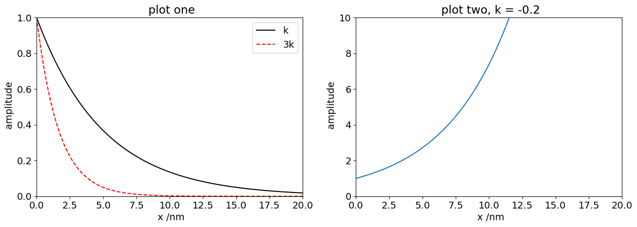
14 Drawing two or more plots#
In this case it is necessary to define a figure and axes rather than using plt as for just a single graph. Using a figure also allows the plot size to be defined rather than having to use the default.
# define an inline (lambda) function
# define a figure  call it fig1 : ( I'm being really imaginative here). We can also define the total size for both figs.

fig1= plt.figure(figsize=(15.5, 10.5))
ax0 = fig1.add_subplot(2,2,1)           # the numbers mean form a 2 x 2 plot and call ax0 and then first plot.
ax1 = fig1.add_subplot(2,2,2)           # etc second plot.
# ax2 = fig1.add_subplot(2,2,4)         # if you remove hash then three plots are drawn

# the notation on subplot is not very clear!
# to draw 4 plots in a square use (2,2,1) (2,2,2), (2,2,3) & (2,2,4)
# if only two axes are defined then only two are drawn; others are left blank
# the way the title limits etc are used is different when subplots are used.

f01 = lambda x, k : np.exp(-k*x)         # define function and make variables x and k.

print('function with x=2 & k=5, is ', f01(2.0,5.0))              # evaluate with x=2, k=5 , note that we used curved brackets for a function

numx = 300
maxx = 20
x = np.linspace(0,maxx,numx)         # numx points in range 0 to maxx

k = 0.2

ax0.plot(x,f01(x,k),color='black',label='k')           # plot whole function on range x with k=0.02
ax0.plot(x,f01(x,3*k),color='red',linestyle='dashed',label='3k')
ax0.set_xlim([0,20])              # notice that we use set_ etc here compared to plt.xlim for just one graph
ax0.set_ylim([0,1])
ax0.set_title(' plot one')
ax0.set_xlabel(' x /nm')
ax0.set_ylabel(' amplitude')
ax0.legend()                     # a peculiarity here as its defined differently to others

k = -0.2
ax1.plot(x,f01(x,k))             # plot whole function on range x with k=-0.02
ax1.set_xlim([0,20])             # notice that we use set_ etc here compared to plt.xlim for just one graph
ax1.set_ylim([0,10])
ax1.set_title(' plot two, k = '+ str(k))   # str(k) makes a string and adds it to previous string in quotes.
ax1.set_xlabel(' x /nm')
ax1.set_ylabel(' amplitude')

plt.show()                       # last plot statement note that this is plt. not an axis.
function with x=2 & k=5, is 4.5399929762484854e-05
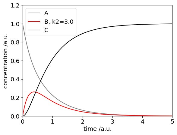
15 Numerical integration of differential equations#
As an example the scheme \(A \leftrightharpoons B \rightarrow C \) is integrated. This is then done algebraically using SymPy in lower down in the document.
The equations are
and the initial conditions at \(t=0\) are \(A[0] = X_0, \; B[0] = 0.0, \; C[0] = 0.0\) where \(X_0\) is defined in the code as the initial amount of A present.
The method by which to do this is shown in the code. (For clarity the reverse rate constant is now called km1 instead of \(k_{-1}\))
from scipy.integrate import odeint    # import odeint used for numerical integration of differential equations

dAdt= '-k1*A + km1*B'                 #  rate equations,put as strings so will not evaluate until variables defined
dBdt= '+k1*A -(km1+k2)*B'
dCdt= '+k2*B'

print('{:s}{:s}\n{:s}{:s}\n{:s}{:s}'.format('dAdt =',dAdt,'dBdt =',dBdt,'dCdt =',dCdt))

k1 = 2.0                                #  rate const A
km1= 1.0                                #  rate const back to A
k2 = 3.0                                #  C does not decay only forms from B

X0 = [1.0, 0.0, 0.0]                    # initial conditions: A, B, C  concentrations

def dX_dt(X, t, const):                 # returns rates dS/dt, dG/dt, dN/dt add extra terms here if necessary
    k1, km1, k2 = const                 # constants needed for calc'n
    A = X[0]                            # X[0] values of A, B ,C which are defined in equations dAdt etc.
    B = X[1]
    C = X[2]
    f = np.array([ eval(dAdt), eval(dBdt), eval(dCdt)])    # make list;  could be f=[eval(dAdt,...)]
                                                           # but numpy is faster
    return f

# do calculation here

maxt = 5.0
numt = 500                                      # number of time points

const =[  k1, km1, k2]                          # constants for calc'n, must be defined bedore here
t = np.linspace( 0, maxt,  numt )               # time as initial, final, then number of points in array

soln = odeint(dX_dt, X0, t, args=(const,) )     # solve equations

Aval, Bval , Cval = soln.T                      # extract results data the .T make the transpose

plt.plot(t,Aval,linestyle='-',color='gray',label='A')
plt.plot(t,Bval,color='red',label='B, k2='+str(k2) )
plt.plot(t,Cval,color='black',label='C')
plt.ylim([0,1.2])
plt.xlim([0,maxt])
plt.xlabel('time /a.u.')
plt.ylabel('concentration /a.u.')
plt.legend()

#plt.savefig('abc-fig1.png')                    # save figure as png; this will overwrite same name
plt.show()
dAdt =-k1*A + km1*B
dBdt =+k1*A -(km1+k2)*B
dCdt =+k2*B
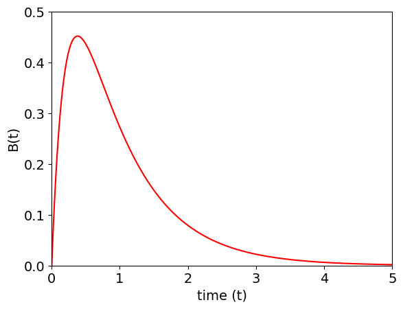
15.1 Algebraic solution using SymPy#
The equations are
and to solve these it is easy to substitute one expression into the other before using the computer and so make a second order equation. C can be obtained from the conditions that if \(A_0\) is the initial amount \(A_0= A_t + B_t + C_t \) after we have found \(A_t, B_t\).
Differentiating B gives
and substituting for \(dA/dt\) and A so that only terms in B remain
Using SymPy the method is shown below. First define the symbols then a function B and the equation.
k1, k2, km1,t = symbols(' k1, k2, km1, t')

B = Function('B')               # unknown function B has t as variable
de= Derivative(B(t),t,t) + (k1+k2+km1)*Derivative(B(t),t) + k1*k2*B(t)
s = dsolve(de )
s
#print(s)

Because constants are produced it is necessary to evaluate these before any further calcuation. At \(t =0\) as \(B =0\) then \(C_1+C_2=0\) and as the total magnitude of the signal does not matter we can set \(C_1=1\) and \(C_2=-1\). The plot below shows the algebraic solution for \(B\).
k1 = 2.0                                #  rate const A
km1= 1.0                                #  rate const back to A
k2 = 3.0                                #  C does not decay only forms from B

maxt= 5.0
numt= 500                                       # number of time points
t = np.linspace( 0, maxt,  numt )               # time as initial, final, then number of points in array
f01= lambda t: -np.exp(t*(-k1 - k2 - km1 - np.sqrt(k1**2 - 2*k1*k2 + 2*k1*km1 + k2**2 + 2*k2*km1 + km1**2))/2) \
               +np.exp(t*(-k1 - k2 - km1 + np.sqrt(k1**2 - 2*k1*k2 + 2*k1*km1 + k2**2 + 2*k2*km1 + km1**2))/2)

plt.plot(t,f01(t),color='red')
plt.xlabel('time (t)')
plt.ylabel('B(t)')
plt.axis([0,5,0,0.5])

plt.show()
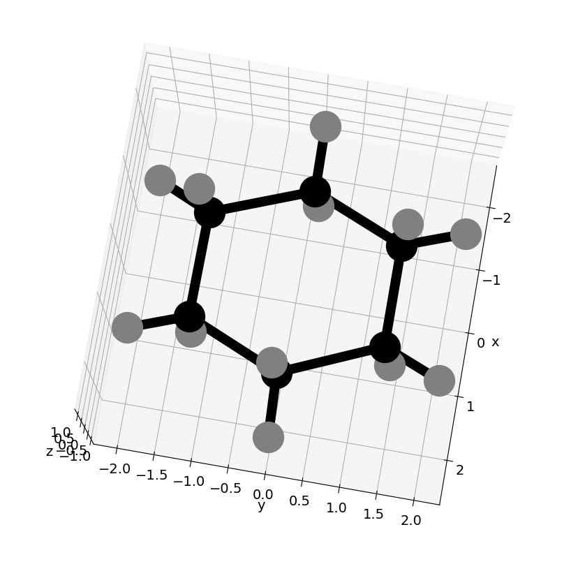
16 Reading data from files and make a 3D plot from .sdf data#
Python has several different ways of reading data and NumPy has even more sophisticated methods. The best way to start with is to use the script with open() as f: as shown below as this automatically closes the file . Use f.readlines() get the whole lot of the data. It reads a list so can be text, numbers or a mixture; it is up to you to sort this out later on.
The example reads an .sdf file. The first 4 lines are header, line 4 contains the number of atoms and number of connections and this is followed by x y z & atom symbol and then the connections list. If there are many lines of data the number of atoms and connections can merge so it is necessary to specifically look for this and correct for it.
# code to read .sdf data and plot 3D graph, xyz contains the coordinates and conect the atom connection list.
# jupyter cannot animate or move graphs easly if at all

dataname = 'cyclohexane.sdf'                                    # put in same folder as notebook as path is not shown
print('{:s}{:s}'.format('Reading sdf data = ', dataname))

with open(dataname,'r') as f:                                   # follow this style using with open() etc.
    data = f.readlines()                                        # readlines reads all file & makes list of strings

num = len(data)
print( '{:d} {:s}'.format(num, ' lines read' ) )


temp = data[3].split()                                          # split data line number 4 as this contains atom numbers
astr = temp[0]
n = len(astr)
if n > 3:                                                       # max number of atoms is 999, and 999 for connections.
    numxyz= int(astr[0:n//2])                                   # note integer division
    numc=   int(astr[n//2:n])
else:
    numxyz= int(temp[0])
    numc =  int(temp[1])
print('{:s}{:4d}{:s}{:4d}'.format('number of atoms =', numxyz, ' number of connections =', numc))

xyz=    [[0.0 for i in range(3)] for j in range(numxyz)]        # coordinates  xyz[j][i]
atm=     ['z' for i in range(numxyz)]                           # atom names
conect= [[  0 for i in range(3)] for j in range(numc)]          # conections

for i in range(numxyz):
    temp = data[i + 4].split()                                  # split list at spaces (default)
    atm[i] = temp[3]                                            # atom symbol in posn 4 e.g Hg, Cl, O etc.
    for j in range(3):
        xyz[i][j]= float(temp[j])                               # x, y z cordinates

for i in range(numc):
    temp = data[i + numxyz + 4].split()
    if len(temp) == 2 :                                         # should be 3 numbers but two may combine
        astr = temp[0]                                          # 1 23 2 if small else 234567 2 if large.
        n = len(astr)
        conect[i][0]= int(astr[0:n//2])
        conect[i][1]= int(astr[n//2:n])
        conect[i][2]= int(temp[1])
    else:
        conect[i][0]= int(temp[0])
        conect[i][1]= int(temp[1])
        conect[i][2]= int(temp[2])

from mpl_toolkits.mplot3d import Axes3D       # make #D plot
fig = plt.figure(figsize=(10.5, 10.5))

ax = fig.add_subplot(111, projection='3d')

adict = {'C':'black', 'O':'red', 'N':'blue', 'S':'yellow', 'H':'gray'}     # dictionary { key1: index1, key2: index2,....}

for i in range(numxyz):
    col='purple'
    if atm[i] in adict:
        col = adict[atm[i]]                                                 # use colour if in dictionary else purple
    ax.scatter(xyz[i][0],xyz[i][1],xyz[i][2], marker='o',color = col, s=1000)
    pass

for i in range(numc):
    indxa = conect[i][0]-1         # -1 because list index starts at zero
    indxb = conect[i][1]-1
    ax.plot([xyz[indxa][0], xyz[indxb][0]],[xyz[indxa][1], xyz[indxb][1]],zs=[xyz[indxa][2], xyz[indxb][2]] ,color='black',linewidth=10)
    pass

ax.set_ylabel('y')
ax.set_xlabel('x')
ax.set_zlabel('z')

ax.view_init(azim=10, elev=80)     # set view angles
pass

plt.show()

# if you use %matplotlib notebook instead of %matplotlib inline you can rotate image etc.
Reading sdf data = cyclohexane.sdf
43  lines read
number of atoms =  18 number of connections =  18
16.1 Reading pdb data#
The code below finds the number of atoms and produces a list of coordinates. Put the .pdb into the same folder as this notebook
dataname='4c3c.pdb'                         # Download data from Brookhaen site https://www.rcsb.org/
print( '{:s} {:s}'.format('filename is ', dataname) )

def get_num_atoms(astr):                    # find string and parse to get number of atoms,
    if line.find(astr) != -1:               # look for 'astr' in whole line; if not there find returns -1
        vals  =line.split()                 # split at spaces
        print('looking for number of atoms ',vals)
        return int(vals[5])                 # from format on pdf must be number in pos'n 5 (counting from 0)
    else:
        return 0                            # not found

numatm = 0
with open(dataname) as f:                   # read lines one at a time
    for line in f:
        numatm = numatm + get_num_atoms('PROTEIN ATOMS')
        numatm = numatm + get_num_atoms('HETEROGEN ATOMS')
        numatm = numatm + get_num_atoms('SOLVENT ATOMS')
    pass
f.close() # not necesary but for clarity

print( '{:s} {:d}'.format('number of atoms is ',numatm))

coords= np.zeros( (numatm,3), dtype=float)               # use numpy to define a numatm by 3 list filled with zeros
atm=  ['' for i in range(numatm)]                        # define an array
cindx=['' for i in range(numatm)]
atyp= ['' for i in range(numatm)]

# now having found number of atoms go back and read data. This saves reading whole file in one go
print('atom       index  separation (Angstrom)      Atom type')
j = 0
with open(dataname) as f:
    for line in f:
        vals = line.split()
        if (vals[0] == 'ATOM') or (vals[0] == 'HETATM'):
            if len(vals[2])  > 4:
                vals.insert(2,vals[2])
            if len(vals[4]) == 5:
                vals.insert(5,vals[4])
            coords[j,0] = float(vals[6])                    # make string into real number
            coords[j,1] = float(vals[7])
            coords[j,2] = float(vals[8])
            atm[j]=   vals[11]
            cindx[j]= vals[1]
            atyp[j]=  vals[2] + ' ' + vals[3]
            #print('{:8s} {:4d} {:12.6f} {:12.6f} {:12.6f}   {:10s}'.format( vals[0], int(vals[1]), float(vals[6]), float(vals[7]), float(vals[8]), vals[11]))

            j=j+1
    pass
filename is  4c3c.pdb
looking for number of atoms  ['REMARK', '3', 'PROTEIN', 'ATOMS', ':', '1549']
looking for number of atoms  ['REMARK', '3', 'HETEROGEN', 'ATOMS', ':', '10']
looking for number of atoms  ['REMARK', '3', 'SOLVENT', 'ATOMS', ':', '165']
number of atoms is  1724
atom       index  separation (Angstrom)      Atom type
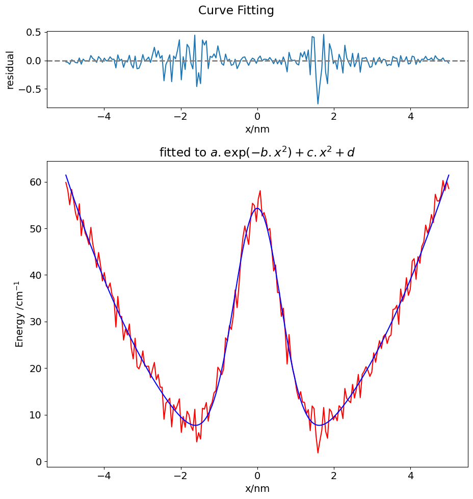
17 Fitting data using non-linear least squares#
In the example below some noisy data is read then, with a function that is supposed to fit the function, the data is analysed. Graphs are plotted.
from scipy.optimize import curve_fit
from matplotlib import gridspec                                     # get this to force size of graphs

fig1= plt.figure(figsize=(8.5, 9))
fig1.suptitle('Curve Fitting')
gs = gridspec.GridSpec(2, 1,width_ratios=[1],height_ratios=[1,4])   # make plots different sizes
ax1 = fig1.add_subplot(gs[0])
ax0 = fig1.add_subplot(gs[1])

eqn = r'$a.\exp(- b.x^2) + c.x^2 + d$'                              #  eqn can be printed out on graph

fit_func = lambda x, a, b, c, d : a*np.exp(- b*x**2) + c*x**2 + d
                                        # must know type of function to fit to, eval makes string into code
                                        # double well potential, gaussian in parabola
# now read in data

dataname = 'data-to-fit.txt'                          # put in same folder as notebook as path is not shown
print('{:s}{:s}'.format('Reading data, filename used is  ', dataname))

with open(dataname,'r') as f:                         # follow this style using with open() etc.
    temp = f.readlines()                              # readlines reads all file & makes list of strings

num = len(temp)
print( '{:4d} {:s}'.format(num, ' lines read' ) )

signal= np.zeros(num,dtype=float)
tme   = np.zeros(num,dtype=float)

for i in range(num):
    f01=  temp[i].split()                             # split line and get two values t and signal
    tme[i]= float(f01[0])
    signal[i]= float(f01[1])
    pass

inits = [10.5, 1.0, 20.0, 10.0]                       # initial values, need not be used in curve_fit

fitP, fitC = curve_fit(fit_func, tme, signal, p0 = inits)  # fitP are parameters, a,b,c,d , fitC are covariances

print('{:s} {:6.3f} {:6.3f} {:6.3f} {:6.3f}'.\
      format('parameters are\n   a       b       c    d\n', fitP[0],fitP[1],fitP[2],fitP[3]))

print('Covarience Matrix \n')
for i in range(4):
    print(fitC[i][:])

the_fit = fit_func(tme,fitP[0],fitP[1],fitP[2],fitP[3])

resid=[ (signal[i]-the_fit[i])/the_fit[i] for i in range(num)]

print('\n{:s}{:8.3g}'.format('Normalised total residual squared ', sum(resid[i]**2 for i in range(num))/num))

ax0.plot(tme,signal,color='red')
ax0.plot(tme,the_fit,color='blue')
ax0.set_xlabel('x/nm')
ax0.set_ylabel('Energy /cm'+r'$^{-1}$')
ax0.set_title('fitted to '+eqn)


ax1.plot(tme,resid)
ax1.axhline(0,color='grey',linestyle='dashed',linewidth=2)
ax1.set_xlabel('x/nm')
ax1.set_ylabel('residual')

fig1.tight_layout()
plt.show()
Reading data, filename used is  data-to-fit.txt
 200  lines read
parameters are
   a       b       c    d
 55.017  1.278  2.485 -0.701
Covarience Matrix

[ 0.41936546  0.00318249  0.00789851 -0.12121503]
[ 0.00318249  0.00147218 -0.00056136  0.00917061]
[ 0.00789851 -0.00056136  0.00083975 -0.01018475]
[-0.12121503  0.00917061 -0.01018475  0.15947232]

Normalised total residual squared   0.0228
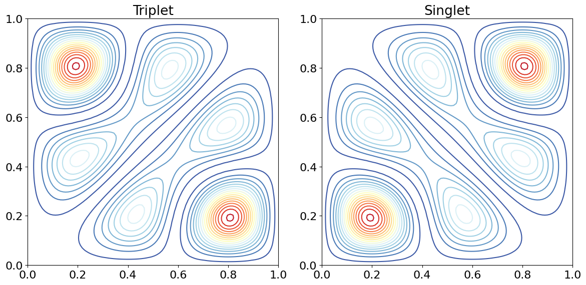
# example of contour plotting for 2D particle in a box spatial wavefunctions

fig1= plt.figure(figsize=(12, 6))
plt.rcParams.update({'font.size': 16})  # set font size for plots, alter at will.

ax0 = fig1.add_subplot(1,2,1)           # 1 row 2 cols in plot then ax0 is plot 1.
ax1 = fig1.add_subplot(1,2,2)
L = 1
n = 2
m = 3

num = 100
f = lambda n,x: np.sqrt(2/L)*np.sin(n*np.pi*x/L)  # wavefunction, qnum n at position x

xa = np.linspace(0,1,num)
xb = np.linspace(0,1,num)

psiT = np.zeros((num,num),dtype=float )
psiS = np.zeros((num,num),dtype=float )

Xa,Xb = np.meshgrid(xa,xb)              # always make grid to do contour plot

for i in range(num):
    for j in range(num):
        psiT[i,j]= 1-( f(n, Xa[i,j] )*f(m,Xb[i,j]) - f( n,Xb[i,j] )*f(m,Xa[i,j]) )**2
        psiS[i,j]= 1-( f(n, Xa[i,j] )*f(m,Xb[i,j]) + f( n,Xb[i,j] )*f(m,Xa[i,j]) )**2

cmap = plt.cm.RdYlBu                      # color map
ax0.contour(Xa,Xb,psiT,cmap=cmap,levels=20)
ax0.set_title('Triplet')
ax1.contour(Xa,Xb,psiS,cmap=cmap,levels=20)
ax1.set_title('Singlet')
plt.tight_layout()
plt.show()
18 Data needed for examples above#
‘data-to-fit.txt’#
remove # after copying
#-5.0             59.854289812
#-4.94974874372   58.1802931927
#-4.89949748744   55.0711715581
#-4.84924623116   58.3405861257
#-4.79899497487   56.0883076321
#-4.74874371859   53.3290150733
#-4.69849246231   51.7838064825
#-4.64824120603   55.2710503925
#-4.59798994975   48.4442916828
#-4.54773869347   51.8376658613
#-4.49748743719   49.0465127074
#-4.4472361809    48.0187755942
#-4.39698492462   46.5301322942
#-4.34673366834   50.2059520632
#-4.29648241206   46.6593203961
#-4.24623115578   44.5577461333
#-4.1959798995    41.6161183466
#-4.14572864322   44.8301013032
#-4.09547738693   42.1573300155
#-4.04522613065   38.7209975092
#-3.99497487437   40.5125772313
#-3.94472361809   37.6602429204
#-3.89447236181   37.150204681
#-3.84422110553   38.2822017573
#-3.79396984925   35.746126679
#-3.74371859296   34.8758613307
#-3.69346733668   28.840409984
#-3.6432160804    35.4019138298
#-3.59296482412   31.1633225852
#-3.54271356784   31.0986435562
#-3.49246231156   26.0433200376
#-3.44221105528   28.4339630025
#-3.39195979899   27.1203947211
#-3.34170854271   29.4839678762
#-3.29145728643   24.3877353808
#-3.24120603015   22.0094501915
#-3.19095477387   26.4406972715
#-3.14070351759   20.3370890653
#-3.09045226131   19.8680580507
#-3.04020100503   21.1385503497
#-2.98994974874   23.706714962
#-2.93969849246   20.4554585086
#-2.88944723618   20.3914079471
#-2.8391959799    20.4418840237
#-2.78894472362   17.9712929447
#-2.73869346734   19.7075282977
#-2.68844221106   21.2352734198
#-2.63819095477   17.542482082
#-2.58793969849   18.667330437
#-2.53768844221   15.9276238272
#-2.48743718593   15.9312428108
#-2.43718592965   9.06098812742
#-2.38693467337   12.5254700504
#-2.33668341709   12.9622476284
#-2.2864321608    13.5685396723
#-2.23618090452   7.41425227714
#-2.18592964824   12.1667037172
#-2.13567839196   11.0931916497
#-2.08542713568   12.1111484718
#-2.0351758794    13.4308647198
#-1.98492462312   6.23366307584
#-1.93467336683   9.64816859361
#-1.88442211055   7.33582779723
#-1.83417085427   10.7674491214
#-1.78391959799   9.99187349798
#-1.73366834171   7.58676502227
#-1.68341708543   6.64575672598
#-1.63316582915   11.178297747
#-1.58291457286   4.20474298874
#-1.53266331658   6.1709410021
#-1.4824120603    4.79668508141
#-1.43216080402   11.4000667759
#-1.38190954774   11.2258541808
#-1.33165829146   12.6423644585
#-1.28140703518   8.66266769899
#-1.23115577889   11.7829956142
#-1.18090452261   12.649888449
#-1.13065326633   14.7285848384
#-1.08040201005   15.2164985858
#-1.03015075377   20.2135801278
#-0.97989949748   19.5302077452
#-0.92964824120   18.5952356839
#-0.87939698492   19.873007487
#-0.82914572864   26.5176183784
#-0.77889447236   25.8641839604
#-0.72864321608   29.1445431593
#-0.67839195979   28.3252900443
#-0.62814070351   31.1448859384
#-0.57788944723   36.7784493969
#-0.52763819095   32.9978347324
#-0.47738693467   37.9428026532
#-0.42713567839   43.8161937415
#-0.37688442211   47.9485495086
#-0.32663316582   50.5189699383
#-0.27638190954   48.4301392223
#-0.22613065326   46.5524869229
#-0.17587939698   51.971823943
#-0.12562814070   55.373996853
#-0.07537688442    54.889888555
#-0.02512562814    51.476646515
#0.025125628140   56.3144958669
#0.075376884422   58.0827899632
#0.125628140704   52.6566776805
#0.175879396985   53.3848239047
#0.226130653266   51.952833851
#0.276381909548   49.5291849722
#0.326633165829   49.9880743129
#0.376884422111   45.5874144944
#0.427135678392   40.862851594
#0.477386934673   42.1461871315
#0.527638190955   36.2426814817
#0.577889447236   36.2412379181
#0.628140703518   31.1194568745
#0.678391959799   32.8747928811
#0.72864321608    27.7905465353
#0.778894472362   20.9116561963
#0.829145728643   27.2232959121
#0.879396984925   22.0091818428
#0.929648241206   19.6359338559
#0.979899497487   17.8808131284
#1.03015075377    15.1549845315
#1.08040201005    13.4078832391
#1.13065326633    14.9723092915
#1.18090452261    12.7402820072
#1.23115577889    12.6779642908
#1.28140703518    10.2130039923
#1.33165829146    11.121922211
#1.38190954774    6.60769521041
#1.43216080402    11.9067562193
#1.4824120603     11.338550556
#1.53266331658    5.61432274929
#1.58291457286    1.84320695013
#1.63316582915    4.40329597508
#1.68341708543    6.64204976519
#1.73366834171    11.5708199553
#1.78391959799    6.46697489345
#1.83417085427    4.97813041772
#1.88442211055    11.266523161
#1.93467336683    10.6697806791
#1.98492462312    8.93040002748
#2.0351758794     9.86409854585
#2.08542713568    8.72359819561
#2.13567839196    11.9506496205
#2.18592964824    11.4445941924
#2.23618090452    9.19973600429
#2.2864321608     15.650912152
#2.33668341709    13.4897125212
#2.38693467337    13.0278794093
#2.43718592965    12.6098245829
#2.48743718593    16.5277197273
#2.53768844221    13.6027091977
#2.58793969849    15.5324221186
#2.63819095477    18.6648580176
#2.68844221106    13.7003463854
#2.73869346734    18.6656340432
#2.78894472362    19.3472468302
#2.8391959799     20.3302568155
#2.88944723618    19.5202958812
#2.93969849246    18.2578750013
#2.98994974874    19.168689628
#3.04020100503    23.2991267427
#3.09045226131    21.2784084146
#3.14070351759    23.8640500851
#3.19095477387    25.9162003493
#3.24120603015    24.2302051946
#3.29145728643    26.7597179616
#3.34170854271    27.2784154976
#3.39195979899    25.3069253354
#3.44221105528    26.7676958713
#3.49246231156    27.133221984
#3.54271356784    32.5926928722
#3.59296482412    32.73068346
#3.6432160804     33.4938973905
#3.69346733668    29.4353395652
#3.74371859296    36.9805795308
#3.79396984925    34.3432884545
#3.84422110553    35.515022334
#3.89447236181    39.4051325332
#3.94472361809    35.6274831293
#3.99497487437    36.9373145527
#4.04522613065    42.9629094387
#4.09547738693    43.4929933753
#4.14572864322    39.0826673714
#4.1959798995     43.930284497
#4.24623115578    42.5180750801
#4.29648241206    46.1452849314
#4.34673366834    47.0994754514
#4.39698492462    50.7107095921
#4.4472361809     48.9955359405
#4.49748743719    50.3015684439
#4.54773869347    52.9586025834
#4.59798994975    51.2565384742
#4.64824120603    57.3076705298
#4.69849246231    55.8909899002
#4.74874371859    55.8806209266
#4.79899497487    57.0427863293
#4.84924623116    60.2637609232
#4.89949748744    58.1114070291
#4.94974874372    60.0270837023
#5.0              58.5432052976
‘cyclohexane.sdf’#
copy and paste the parts needed but remove any #
#test CX
#  --CCDC--102811    3D
#
# 18 18  0  0  0  0  0  0  0  0999 V2000
#    0.7430   -1.2880   -0.2703  C     0
#    1.4588   -0.0216    0.2583  C     0
#    0.7158    1.2663   -0.1544  C     0
#   -0.7158    1.2623    0.2638  C     0
#   -1.4392    0.0337   -0.2382  C     0
#   -0.7430   -1.2407    0.1609  C     0
#    0.7629   -1.3083   -1.2361  H     0
#    2.3504    0.0027   -0.0975  H     0
#    1.5238   -0.0680    1.2151  H     0
#    0.7656    1.3748   -1.1069  H     0
#    1.1552    2.0183    0.2502  H     0
#   -1.1471    2.0491   -0.0786  H     0
#   -0.7681    1.2892    1.2222  H     0
#   -1.4997    0.0758   -1.1952  H     0
#   -2.3317    0.0318    0.1141  H     0
#   -0.7939   -1.3433    1.1144  H     0
#   -1.2072   -1.9810   -0.2378  H     0
#    1.1386   -2.0189    0.0411  H     0
#  2  1  1
#  3  2  1
#  4  3  1
#  5  4  1
#  6  1  1
#  6  5  1
#  7  1  1
#  8  2  1
#  9  2  1
# 10  3  1
# 11  3  1
# 12  4  1
# 13  4  1
# 14  5  1
# 15  5  1
# 16  6  1
# 17  6  1
# 18  1  1
#M  END
#$$$$
Chapter 11 Q20#
‘UK-covid-deaths.txt’#
This is a text file. Note that the data is in reverse order so will need to be reversed before using. If the data is read into \(\mathtt{alldata[\,:\,]}\), then \(\mathtt{revdata[\,:\,]=alldata[\,:\,:\,-1]}\) will reverse it.
160545, 160463, 160356, 160235, 160097, 159967, 159832, 159704, 159551, 159402, 159241, 159077, 158898, 158703, 158527, 158312, 158088, 157836, 157596, 157357, 157099, 156846, 156549, 156288, 156048, 155767, 155516, 155238, 154932, 154679, 154400, 154119, 153827, 153537, 153245, 152973, 152689, 152435, 152169, 151891, 151624, 151385, 151135, 150881, 150669, 150451, 150273, 150096, 149916, 149748, 149558, 149434, 149265, 149125, 149008, 148905, 148778, 148647, 148521, 148421, 148298, 148197, 148089, 147961, 147855, 147744, 147615, 147513, 147393, 147298, 147193, 147068, 146956, 146835, 146697, 146586, 146440, 146311, 146204, 146079, 145983, 145860, 145742, 145635, 145503, 145366, 145250, 145108, 144990, 144885, 144755, 144631, 144495, 144369, 144217, 144043, 143917, 143782, 143633, 143490, 143342, 143193, 143037, 142871, 142703, 142545, 142389, 142224, 142066, 141889, 141701, 141532, 141361, 141168, 141007, 140843, 140710, 140558, 140393, 140257, 140099, 139945, 139817, 139690, 139561, 139428, 139289, 139140, 139020, 138905, 138780, 138684, 138567, 138447, 138324, 138221, 138101, 137998, 137902, 137792, 137663, 137550, 137425, 137317, 137201, 137104, 136979, 136854, 136715, 136564, 136443, 136306, 136181, 136058, 135881, 135730, 135585, 135431, 135321, 135178, 135040, 134894, 134728, 134587, 134432, 134293, 134136, 134002, 133855, 133726, 133608, 133492, 133385, 133256, 133130, 133003, 132887, 132785, 132671, 132556, 132437, 132331, 132214, 132105, 132003, 131893, 131809, 131722, 131626, 131519, 131412, 131324, 131243, 131162, 131082, 130987, 130893, 130791, 130711, 130637, 130556, 130461, 130371, 130265, 130184, 130096, 130024, 129948, 129876, 129803, 129720, 129643, 129588, 129530, 129448, 129381, 129329, 129277, 129225, 129182, 129132, 129091, 129057, 129015, 128968, 128926, 128897, 128864, 128835, 128806, 128777, 128749, 128724, 128703, 128679, 128666, 128644, 128627, 128605, 128582, 128574, 128561, 128545, 128520, 128497, 128485, 128479, 128466, 128445, 128435, 128425, 128411, 128405, 128394, 128385, 128375, 128369, 128361, 128354, 128342, 128330, 128317, 128313, 128305, 128296, 128287, 128279, 128270, 128257, 128250, 128241, 128232, 128228, 128219, 128213, 128208, 128202, 128194, 128186, 128178, 128172, 128165, 128154, 128139, 128129, 128120, 128111, 128099, 128089, 128076, 128066, 128056, 128042, 128033, 128021, 128006, 127990, 127975, 127961, 127946, 127938, 127915, 127898, 127874, 127855, 127837, 127819, 127794, 127776, 127754, 127737, 127716, 127687, 127663, 127638, 127612, 127576, 127548, 127520, 127502, 127475, 127444, 127413, 127381, 127343, 127300, 127264, 127230, 127191, 127143, 127097, 127056, 127004, 126937, 126856, 126792, 126722, 126664, 126584, 126501, 126406, 126309, 126201, 126109, 125985, 125867, 125730, 125586, 125453, 125301, 125132, 124978, 124831, 124647, 124423, 124211, 123981, 123753, 123493, 123218, 122929, 122647, 122321, 121969, 121589, 121171, 120740, 120293, 119775, 119279, 118788, 118254, 117678, 117069, 116458, 115779, 115142, 114440, 113687, 112968, 112110, 111257, 110361, 109466, 108553, 107484, 106374, 105260, 104195, 103026, 101867, 100696, 99451, 98213, 96914, 95550, 94253, 92983, 91672, 90444, 89214, 87995, 86782, 85651, 84553, 83530, 82543, 81547, 80613, 79704, 78859, 78099, 77337, 76587, 75829, 75107, 74447, 73768, 73110, 72453, 71838, 71254, 70688, 70124, 69549, 69043, 68554, 68039, 67501, 67069, 66608, 66129, 65710, 65272, 64819, 64371, 63939, 63503, 63078, 62657, 62262, 61786, 61311, 60924, 60525, 60101, 59635, 59164, 58738, 58304, 57816, 57352, 56888, 56411, 55944, 55490, 55028, 54539, 54095, 53672, 53217, 52783, 52346, 51925, 51534, 51143, 50659, 50244, 49850, 49448, 49068, 48739, 48377, 48038, 47678, 47353, 47013, 46699, 46412, 46144, 45863, 45611, 45398, 45174, 44938, 44717, 44517, 44325, 44164, 43985, 43835, 43684, 43567, 43456, 43343, 43218, 43114, 43034, 42939, 42837, 42766, 42694, 42634, 42567, 42498, 42431, 42374, 42326, 42272, 42223, 42184, 42151, 42116, 42059, 42019, 41992, 41960, 41940, 41916, 41888, 41861, 41843, 41822, 41805, 41787, 41774, 41761, 41751, 41741, 41726, 41717, 41704, 41695, 41685, 41675, 41670, 41660, 41654, 41649, 41638, 41629, 41618, 41606, 41600, 41584, 41575, 41568, 41560, 41556, 41547, 41535, 41531, 41519, 41512, 41503, 41496, 41486, 41473, 41464, 41450, 41437, 41428, 41422, 41408, 41392, 41382, 41371, 41357, 41347, 41335, 41323, 41311, 41294, 41277, 41270, 41254, 41236, 41216, 41204, 41190, 41176, 41158, 41145, 41125, 41104, 41079, 41065, 41044, 41022, 40985, 40961, 40934, 40898, 40871, 40838, 40809, 40766, 40739, 40692, 40653, 40608, 40559, 40518, 40450, 40376, 40311, 40247, 40193, 40133, 40081, 40020, 39961, 39877, 39805, 39719, 39656, 39576, 39496, 39387, 39297, 39172, 39044, 38934, 38811, 38677, 38522, 38354, 38219, 38092, 37929, 37743, 37526, 37329, 37115, 36915, 36719, 36499, 36276, 36038, 35770, 35495, 35202, 34935, 34621, 34307, 33973, 33656, 33335, 33026, 32678, 32300, 31917, 31456, 30996, 30531, 30047, 29597, 29103, 28535, 27984, 27412, 26853, 26258, 25625, 24978, 24295, 23617, 22886, 22141, 21358, 20590, 19790, 18971, 18128, 17250, 16393, 15497, 14539, 13583, 12639, 11638, 10562, 9563, 8668, 7751, 6845, 6005, 5199, 4430, 3769, 3179, 2673, 2237, 1839, 1477, 1174, 937, 751, 587, 457, 348, 275, 207, 155, 108, 76, 54, 38, 25, 17, 14, 9, 6, 6, 6, 3, 3, 1
Chapter 13#
‘test data.txt’#
remove # after copying
#200, 36.2, 1.5
#220, 42.7, 1.1
#240, 44.9, 1.8
#260, 51.8, 0.3
#280, 57.7, 2.0
#300, 60.9, 0.9
#320, 64.4, 1.2
#340, 68.2, 1.6
#360, 76.4, 1.9
#380, 80.1, 0.9
‘PCA data.txt’#
remove # after copying
#2.75, 6.00, -0.52
#1.65, 1.75, -0.39
#2.42, 7.25, -0.64
#2.09, 5.50, -1.17
#3.41, 7.50, -1.10
#2.53, 6.75, -0.67
#2.20, 4.00, -1.01
#1.10, 2.75, -0.62
#1.65, 4.00, -1.25
#1.21, 2.25, -0.61
‘exponential-data.txt’#
remove # after copying
# 1 , 1927, 1927
# 5 , 1329, 1329
# 9 , 812 , 812
# 13, 568 , 568
# 17, 390 , 390
# 21, 290 , 290
# 25, 171 , 171
# 29, 112 , 112
# 33, 87  , 87
# 37, 48  , 48
# 41, 43  , 43
# 45, 26  , 26
# 49, 26  , 26
# 53, 14  , 14
# 57, 13  , 13
# 61, 10  , 10
# 65, 6   , 6
# 69, 9   , 9
# 73, 8   , 8
# 77, 7   , 7
# 81, 3   , 3
# 85, 9   , 9
# 89, 5   , 5
# 93, 4   , 4
# 97, 8   , 8