
3.9 Trig functions, logs, power, reciprocals and integrals
Contents
3.9 Trig functions, logs, power, reciprocals and integrals#
# import all python add-ons etc that will be needed later on
%matplotlib inline
import numpy as np
import matplotlib.pyplot as plt
from sympy import *
init_printing()                      # allows printing of SymPy results in typeset maths format
plt.rcParams.update({'font.size': 14})  # set font size for plots
3.9 Differentiating sine and cosine#
Sine and cosine functions are almost mirror images of one another when differentiated,
which makes sense if one inspects a graph of these functions, see Fig. 5. The value of the cosine at any point is the gradient of the sine at that point and the gradient of the cosine is \(-1\) times the value of the sine. When the sine has its maximum or minimum, where the gradient is zero, the value of the cosine is also zero. Furthermore, when the gradient of the sine is positive, \(x/\pi = 0 \to 1/2\) and also \(3/2 \to 2\), the value of the cosine, which is the derivative, is positive. When the gradient of the sine is negative, the value of the cosine is negative. It is therefore not surprising that on differentiating these functions again they turn into one another but with a change of sign depending upon how many times this is done.
the pattern being \( +\cos,\; -\sin,\; -\cos,\; +\sin \cdots\) with the powers of \(a\) increasing each time.
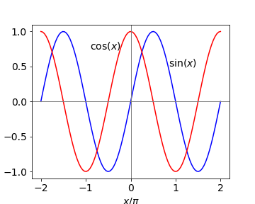
Figure 5. Sine and cosine over two periods.
3.10 Other trig functions, tan, sec and hyperbolic functions sinh, cosh and their inverse.#
There are many other trigonometric and closely related hyperbolic functions besides sine and cosine, and most can be treated by the differentiation methods described in the next few sections based on basic differentiation. One useful way is to convert to the exponential form first. Sine and cosine can easily be differentiated this way, then converted back to a trig form. A tangent, for example, is the ratio of sine/cosine and is treated as a ratio. Others functions such as sec(x) which is 1/cos(x) can be treated as a function of a function, Section 5.1, either in the trig or exponential form. The hyperbolic functions cosh, sinh, and tanh also have exponential representations. The Pythagoras right-angled triangle can also be used to convert between trig functions, see Chapter 1.5.
The inverse functions \(\displaystyle y=\sin^{−1}(x),\; y = \cosh^{-1}(x)\), and so forth can be treated by rearranging the equation, for instance,
and differentiating both sides (see eqn. 6 ), produces, \(\displaystyle \cos(y)\frac{dy}{dx}=2x\) and \(y\) can be substituted into this using \(\displaystyle \cos^2(x)+\sin^2(y)=1\) giving
The final result is
The general case when \(\displaystyle y=\sin^{-1}(ax+b) \) has the differential
and this result and others are given in the table of derivatives in section 3.17.
(i) Rainbows#
In forming a rainbow light is refracted and reflected in raindrops back towards then observer. The angle light returns at relative to the observer is \(\approx 42^\mathrm{o}\) to the sun. The colours are due to the changing refractive index (dispersion) with wavelength, the index being larger at shorter wavelengths. The semicircular nature of the rainbow is due to the cylindrical symmetry about the rays from the sun and if the sun is very low in the sky or you are on a hill, the rainbow can effectively become circular. Descartes first explained the rainbow in circa 1637.
The figure below shows the geometry. The ray enters at A with an incidence angle \(i\) and is refracted by the water droplet at angle \(r\) according to Snell’s law
where \(n\) is the refractive index at the wavelength chosen, for example, \(n=1.3370\) at \(450\) nm and \(1.331\) in the red at \(650\) nm. The ray is totally internally reflected at angle \(r\), the incident. and reflected angles are the same in reflection, and then leaves at C after being refracted again. The total angle between the incident and outgoing ray is \(\displaystyle \theta =4r-2i\), which can be found from straightforward geometry.
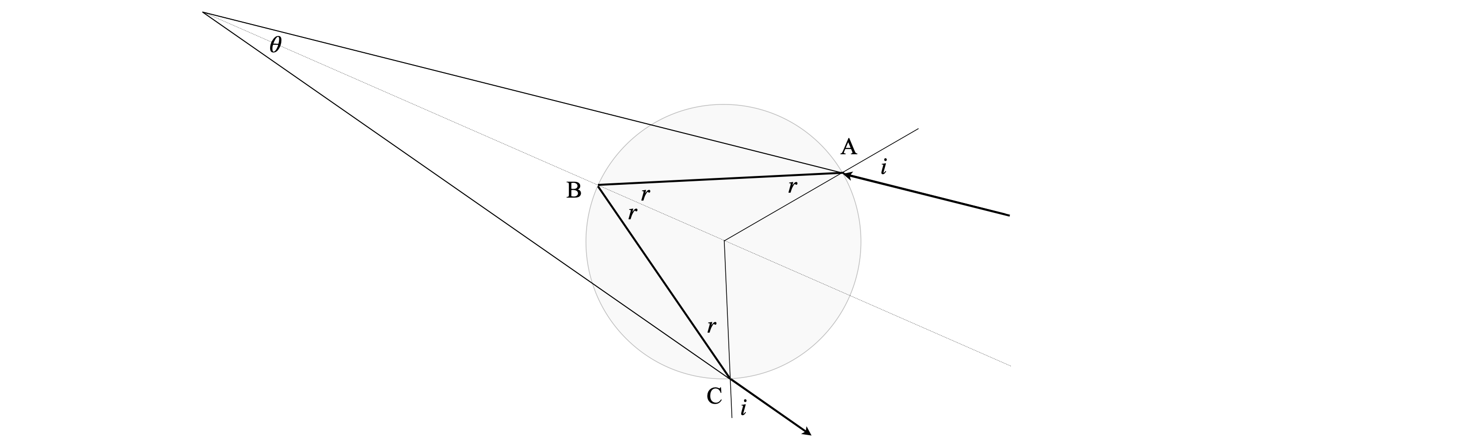
figure 5a. The ray from the sun arriving at A is refracted according to Snell’s Law, totally internally reflected at B and exits the raindrop at C and travels towards the observer’s eye. The angle \(\theta\) is the acute angular change in direction and is labelled \(\theta_R=\approx 42^o\) when a rainbow is observed. Rays entering parallel to that at A (not shown) but do so closer to the centre line also cluster around angle \( \theta_R\) for a given wavelength.
Substituting for Snell’s law produces
where \(\theta\) is a function of the incident angle \(i\). This function has a maximum called the rainbow angle \(\theta_R\) when its derivative is zero. To find the derivative the method above could be used but gives a rather complicated answer. It is better in this case to use the general formula by letting \(ax= sin(i)/n\) and \(b=0\) but remember that you must multiply by the derivative of \( \sin(i)/n\) as in the function of function method. The result is
and the value of \(i\) when the function is at its maximum is found when the derivative is zero, and after some simplification, this is
This value for \(i\) has to be used to find \(\theta_{R}\), which is the minimum deviation angle. At \(450\) nm using the refractive index given above the angle is \(\theta_R = 41.5^\mathrm{o}\) and at \(650\) nm \(42.37^\mathrm{o}\) so red light is scattered through a greater angle than blue light. Although these angle are only slightly different over the distance involved are enough to cause the colours to separate. If the angle \(\theta\) is not about \(42^\mathrm{o}\) then the intensity will be low and no rainbow observed. The geometry of the rain droplet returns light preferentially at angles clustered about \(\theta_R\) and much less over other angles. For example if the sun were high enough to make the angle greater that \(\theta_R\) with respect to the observer no rainbow could be seen.
3.11 Repeated differentiation#
The sine, cosine and exponential functions are capable of endless repeated differentiation as shown in section 3.9. If \(\displaystyle y=e^{-ax}\) differentiating twice produces,
Continuing the differentiation, the powers of \(a\) increase and the sign alternates being positive for even powers and negative for odd ones. The \(n^{th}\) derivative is
which is simply the differential equation
Importantly, this tells us that the solution to equations of this type are exponentials.
3.12 Differentiating logarithms#
In a 1697 paper Johann Bernoulli states ( Dunham 2018),
‘The differential of a logarithm, no matter how composed, is equal to the differential of the expression divided by the expression’
thus differentiating logarithms always has the form:
for example,
Differentiating \(\ln(y)\) with respect to \(x\) produces a most useful form, which is worth remembering
Example (i) The Van’t Hoff equation#
The van’t Hoff equation of chemical thermodynamics has this last form,
This equation describes the change of an equilibrium constant \(K_p\) for a reaction carried out at constant pressure with temperature \(T\) and quantifies the Le Chatelier principle. \(\Delta_rH^{\mathrm{o}}\) is the standard molar enthalpy of the reaction. In this form it is easier to plot or integrate wrt. temperature.
Example (ii)#
A particularly cunning and somewhat complicated example using this log derivative is to solve the equation
where both \(R\) and \(S\) are functions of \(x\). The first step is to divide by \(R\) and then to use the form of equation 11 on the derivative in \(R\).
Now suppose we substitute \(U =dS/dx\) then \(dS^2/dx^2\equiv dU/dx\),
and then divide by \(U\) and use eqn 11, substitute back and simplifying gives
The solution is
where \(C\) is a constant. The reason \(C\) is there is that this is the general form and is simplified from the derivative of a log, since \(\displaystyle \frac{d}{dx}\ln(Cx)=\frac{1}{x}\).
Example (iii) An infinite product#
The product \(\displaystyle \prod_{n=1}^\infty \left(1-\frac{x^2}{n^2}\right)\) cannot be easily differentiated but its log can be and so
and
3.13 Differentiating \(x\) as a power, factorials \(x!\) and absolute values \(|x|\)#
Expressions such as \(y=a^x,\;y=x^{1/x},\; y= x^x \) etc. can be differentiated quite easily with a little care.
(i) \(a^x\)#
In cases where there are powers of \(x\) it is best to take logs of both sides first. For example, if \(y = a^x\), taking logs of both sides gives \(\ln(y) = x \ln(a)\) and differentiating produces
and simplifying produces
In the special case that \(a = e\) (\(e\) is the exponential constant), then the exponential derivative is retrieved because \(\ln(e) = 1\).
(ii) Which is larger \(e^\pi\) or \(\pi^e\) ?#
As a second example we differentiate \(x^{1/x}\) and from this we can determine which is larger \(e^\pi\) or \(\pi^e\) in other words is \(e^\pi >\pi^e\) or not. Taking logs of both side gives \(\pi\ln(e)>e\ln(\pi)\), and dividing by \(e\) and \(\pi\) gives \(\displaystyle \frac{\ln(e)}{e}>\frac{\ln(\pi)}{\pi}\) thus the test to make is to see if \(\displaystyle e^{1/e}>\pi^{1/\pi}\) or not. If the maximum of \(x^{1/x}\) can be found then we determine if the inequality is true or not.
First take logs giving \(\displaystyle \ln(y)=\frac{1}{x}\ln(x)\) and then differentiate and using eqn. 11 to simplify gives
To determine which is bigger \(e^\pi\) or \(\pi^e\) means that we should compare \(e^{1/e}\) and \(\pi^{1/\pi}\). The thing to realize here is that if we find the maximum of the derivative of \(x^{1/x}\) we can then check which of our two terms is bigger. To find the minimum/maximum is very simple (see section 9) and is found by setting the derivative to zero, then \(\ln(x)=1\) so that \(x=e\) is the global maximum and this means that \(e^{1/e}\) is the maximum possible value and so \(e^\pi\; \gt\; \pi^e\). The graph of \(\displaystyle x^{1/x}\) is zero at \(x=0\), rises rapidly then decreases again as \(x\) increases.
(iii) Factorials#
A factorial is defined as \(x!=x\cdot(x-1)\cdot (x-2)\cdots 2\cdot 1\) where \(x\) is an integer, thus this function cannot be differentiated. Factorials occur most commonly in evaluating probabilities such as the binomial coefficients
and sometimes it is necessary to determine the maximum of a distribution containing this term, which thus requires differentiation.
Fortunately, for large \(x\) Stirling’s Rule can be used which is
where \(x\) is assumed not to be an integer but a variable. Differentiating the log produces
To find the maximum in \(\displaystyle \binom{n}{x}\equiv y=\frac{n!}{x!(n-x)!}\),
substitute for the factorials using Stirling’s formula, differentiate and set the result to zero.
substituting for \(y\) produces
and the maximum (or minimum) is found when the derivative is zero which can only be when \(\ln(x)=\ln(n-x)\) or \(x=n/2\). This can only be a maximum because the distribution is always positive and can be confirmed by direct calculation or plotting values. See Pascal’s triangle and Binomial distribution in Chapters 1 and 12.
The derivative of any factorial can be evaluated using the Gamma function (see Chapter 1-8). The Gamma function produces factorials of any number, positive or negative, not just integers. Using \((x-1)!=\Gamma(x)\) the formula for the derivative \(\Gamma'(x)\) is
where \(\gamma=0.57721\dots\) is the Euler-Mascheroni constant.
(iv) Absolute or modulus |x|#
The absolute value or modulus \(|x|\) is defined as positive \(+x\) if \(x\) is either positive or negative or zero if \(x=0\) and can be differentiated by writing it as \(\sqrt{x^2}\) in which case
which is \(\pm 1\) depending on the sign of \(x\). More complicated functions can be treated in the same way
which is \(sign(\sin(x))\cos(x)\).
3.14 Reciprocal derivatives#
Occasionally it is necessary, or simpler, to find \(dx/dy\) rather than invert the equation to put it in terms of \(y = \cdots\) and calculate \(dy/dx\). The derivatives are related as double reciprocals;
As an example, suppose that \(\displaystyle \sin(y^2) = x\), differentiating by \(y\) gives the result \(\displaystyle dx/dy = 2y \cos(y^2)\). Differentiating by \(x\) could mean that a rearrangement must first be done to form \(\displaystyle y = \sqrt{\sin^{-1}(x)}\) and then this differentiated, which is quite involved. Instead using equation (6), the result is obtained directly \(\displaystyle 2y \cos(y^2)dy/dx = 1\) and these two results show that equation (13) is true.
3.15 Differentiating integrals#
If you are unfamiliar with integration, it will help to know the basic rules; see Chapter 4. In that chapter more examples are given particularly using both the Leibniz formula and Feynman’s method of evaluating integrals. Only an outline of differentiating an integral is given here.
Differentiating a definite integral with two limits both of which are constants, i.e. simply numbers \(a\) and \(b\), produces zero, because integration with such limits produces a number, e.g. the area under the curve from \(a\) to \(b\), see Fig. 1, and the differential of a constant is zero,
In the more complex and general case, where the limits \(u\) and \(v\) are themselves functions of \(x\), the function of function rule is used (Section 5.1) as shown next.
The fundamental theorem of the calculus states that
and to differentiate an integral with one limit that is a function of \(x\), i.e. \(v(x)\) and one a constant \(a\) we start with
and let \(y=v(x)\) thus
When both limits are functions
which is the simpler form of Leibniz’s Integral Rule. An example where \(x^2\) is one of the limits is,
The aim in differentiating integrals is not to work out the integral first, which might not be possible anyway, and then differentiate the result, but to use equation (15), which avoids doing this.
3.16 Fractional derivatives#
While it is possible to repeatedly take derivatives of many functions, for instance \(\displaystyle \frac{d^3}{dx^3}\sin(x)\), what about the \(1/3\) or \(1/2\) or \(-1\) derivative? What would such a thing mean? In the case of \(1/2\) derivatives we can say that if the function is \(x^n\) then the half derivative is such that \(\displaystyle \frac{d^{1/2}}{dx^{1/2}}\frac{d^{1/2}}{dx^{1/2}}x^n\equiv nx^{n-1}\). In other words differentiating, or operating twice on \(x^n\) with \(d^{1/2}/dx^{1/2}\), is the same as differentiating once with \(dy/dx\).
The general result for the \(n^{th}\) derivative of \(x^m\) is \(\displaystyle \frac{d^ny}{dx^n}=\frac{m!}{(m-n)!}x^{m-n}\) which can be generalised if \(n\) is a fraction by changing the factorials to gamma functions as \(n!=\Gamma (n+1)\) thus \(\displaystyle \frac{d^ny}{dx^n}=\frac{\Gamma (m+1)}{\Gamma(m-n+1)}x^{m-n}\). As many functions can be expressed as power series it is possible to fractionally differentiate these. However, these unusual derivatives need not have more than a curiosity interest for us; they appear in Morse’s paper on the anharmonic oscillator (P. Morse, Physical Review, 34, 57, 1929) and hardly anywhere else.
3.17 Table of Differentials#
\(a,\;b,\;\) and \(n\) are treated as constants.
Using python/Sympy is very easy for more complex functions.
x,a,b = symbols('x,a,b')

f01 = x**b*sin(a*x)**3
diff(f01,x)
