12 Basis sets with more than three dimensions

12 Many dimensions

The \(x, y\), and \(z\)-axes at \(90^\text{o}\) to one another are very familiar and the basis set of unit vectors \(\boldsymbol i, \boldsymbol j, \boldsymbol k\) can be used to describe any vector in these axes. These basis vectors are orthogonal; geometrically they are each at \(90^\text{o}\) to one another and their dot product is zero. We have seen that \(\boldsymbol i\cdot\boldsymbol j = \boldsymbol j\cdot\boldsymbol k = \boldsymbol i\cdot\boldsymbol k = 0\) and that the vectors are normalized, \(\boldsymbol i\cdot\boldsymbol i = \boldsymbol j\cdot\boldsymbol j = \boldsymbol k\cdot\boldsymbol k = 1\); however, not all of the properties of molecules are represented in three dimensions. For instance, molecular orbitals need large basis sets. Benzene for instance, would need at least a six element basis set just to describe the \(\pi\) electrons alone. At the other extreme, we could have an infinite basis set, which is also quite common in quantum mechanical problems and would be needed to handle the infinite number of vibrational levels in a harmonic oscillator. Fortunately, a large basis set is handled in the same way as a small one.

Suppose a four-dimensional set of unit vectors is made each one lying along one of four orthogonal axes. We cannot represent this geometrically in any easy way, but we can do so algebraically. The simplest way is to make a vector, row or column, containing the four elements and then to normalize it if necessary. In question 28 we used a wavefunction of the form \(\psi = a\psi_s + b\psi_{px} + c\psi_{py} + d\psi_{pz}\). This wavefunction is expressed in the basis set of one 2s and three 2p atomic orbitals \(\psi_s, \psi_{px}, \psi_{py}, \psi_{pz}\). We assume that each of these orbitals are already orthogonal and normalized; i.e. that they form an orthonormal basis set. If they are not orthonormal then we have to perform a Gram - Schmidt orthogonalization procedure, which we need not delve into, but is described in more advanced texts such as Arkfen (1970).

The four-dimensional basis set can be written either as a column or as a row vector, it does not matter which, but the rules for normalization and orthogonality are here assumed to be understood and are not stated explicitly.

\[\displaystyle (\psi_s, \psi_{px}, \psi_{py}, \psi_{pz})\]

In standard column vector notation the basis set is

\[\begin{split}\displaystyle (\psi_s, \psi_{px}, \psi_{py}, \psi_{pz})=\left(\; \begin{bmatrix}1\\0\\0\\0\end{bmatrix},\;\begin{bmatrix}0\\1\\0\\0 \end{bmatrix},\;\begin{bmatrix}0\\0\\1\\0 \end{bmatrix},\;\begin{bmatrix}0\\0\\0\\1 \end{bmatrix}\;\right) \end{split}\]

and the normalization and orthogonality is clear. Wavefunctions describing the eigenstates of a molecule or atom are orthogonal, but not necessarily normalized, and are used to calculate the expectation values of operators. The orbitals \(\psi_{2px}, \psi_{2py}, \psi_{2pz}\) are hybrid orbitals in the basis set of the three 2p orbitals with quantum numbers \(n = 2, l = 1, m = 0, \pm 1\) and are

\[\displaystyle \psi_{2p_x}=\frac{1}{\sqrt{2}}(\psi_{2p_{-1}}+\psi_{2p_{+1}}),\quad \psi_{2p_x}=\frac{i}{\sqrt{2}}(\psi_{2p_{-1}}-\psi_{2p_{+1}}),\quad \psi_{2p_z}=\psi_{2p_0} \]

and as the \(\psi_{2p_{0,\pm 1}}\) functions are known, (they are spherical harmonics), the spatial extent of the wavefunctions, for instance, can be calculated. However, if we change the calculation to one using vectors, many other calculations can more simply be made. In fact, if the wavefunctions were to represent quantum mechanical ‘spin’, such as the spin properties of the electron or of a nucleus, the wavefunction is only known symbolically and a vectorial approach is essential.

Returning to the three 2p orbitals these can equivalently be written as

\[\displaystyle \vec v_{2p_x}=\frac{1}{\sqrt{2}}(\boldsymbol i+\boldsymbol j),\quad \vec v_{2p_x}=\frac{1}{\sqrt{2}}(\boldsymbol i-\boldsymbol j),\quad \psi_{2p_z}=\boldsymbol k\]

in the three-dimensional \(i, j, k\) basis set. In vector form the equations are

\[\displaystyle \vec v_{2p_x}=\frac{1}{\sqrt{2}}\begin{bmatrix}1&1&0\end{bmatrix},\quad \vec v_{2p_y}=\frac{1}{\sqrt{2}}\begin{bmatrix}1&-1&0\end{bmatrix},\quad \vec v_{2p_z}=\frac{1}{\sqrt{2}}\begin{bmatrix}0&0&\sqrt{2}\end{bmatrix}\]

and column vectors would be equally acceptable. A basis set for the s and three 2p orbitals cannot be written using the \(i, j, k\) basis set because there are four elements. A vector must be used and in row-vector form a hybrid orbital of s and a mixture of 2p\(_x\), 2p\(_y\), and 2p\(_z\) orbitals making 2sp\(^2\) hybrid orbitals have combinations

\[\displaystyle \vec v_{1}=\frac{1}{\sqrt{6}}\begin{bmatrix}\sqrt{2}& -1&\sqrt{3}&0\end{bmatrix}, \quad \vec v_{2}=\frac{1}{\sqrt{6}}\begin{bmatrix}\sqrt{2}& -1&-\sqrt{3}&0\end{bmatrix}\]

where the basis set ordering is s, p\(_x\), p\(_y\), p\(_z\). If we are dealing with a conjugated molecule, conventionally the \(z\) direction or 2p\(_z\) orbital is used to form any \(\pi\) bonds, the s and other two 2p orbitals form the sp\(^2\) hybrid, the last entry of the \(\vec v_1\) and \(\vec v_2\) vectors is thus zero. To test if the orbitals are orthogonal, calculate their dot product. (The superscript \(T\) means make the transpose that converts rows into columns or vice versa.)

\[\begin{split}\displaystyle \vec v_1\cdot \vec v_2=[v_1][v_2]^T=\frac{1}{6}\begin{bmatrix}\sqrt{2}&-1&-\sqrt{3}& 0 \end{bmatrix}\begin{bmatrix}\sqrt{2}\\-1\\ \sqrt{3}\\ 0 \end{bmatrix} =(2+1-3+0)/6=0 \end{split}\]

where \([v]\) means vector \(v\). This dot product shows that the two sp\(^2\) orbitals are orthogonal in the basis of the s and the three 2p- atomic orbitals. Each orbital is normalized as \(\vec v_1\cdot \vec v_1 = 1\) and similarly for \(\vec v_2\). Chapter 7 gives the matrix row-column multiplication rules.

13 Large and infinite basis sets

Large basis sets are often, but not always, needed when solving quantum mechanical problems. The basis set will contain \(n\) vectors starting with \(\vec x_1\) and extending up to \(\vec x_n\) instead of just three such as \(i, j, k\). Any vector is written in the usual way as a linear combination of the \(\vec x\) base vectors multiplied with constant coefficients \(v_1 \to v_n\), and we shall assume, for simplicity, that these are scalars, i.e. simple numbers and not complex numbers as they can sometimes be in quantum problems. The basis set vectors are, by definition, orthonormal.

A vector \(\vec V\) is always written as a linear combination of base vectors \(\vec x\),

\[\displaystyle \vec V=v_1\vec x_1+ v_2\vec x_2+v_3\vec x_3+\cdots +v_n\vec x_n =\sum_{p=1}^n w_p\vec x_p \]

and the index \(q\) takes the values from \(1 \to n\). Note that here we will use \(v,\;w\) as coefficients of \(\vec V\) and \(\vec W\) respectively not vectors as in other sections.

Suppose that there is another vector \(\vec W\) then in the same fashion then \(\displaystyle \vec W=\sum_{p=1}^n w_p\vec x_p \) and the dot product is

\[\begin{split}\displaystyle \vec W \cdot \vec V= \left(\sum_{p=1}^n w_p\vec x_p\right)\left( \sum_{q=1}^n v_p\vec x_q\right)\equiv \begin{bmatrix}w_1&w_2&\cdots\end{bmatrix} \begin{bmatrix}v_1\\v_2\\ \vdots\end{bmatrix} \qquad\qquad\qquad\qquad\qquad\qquad\text{(35)}\end{split}\]

in this case, also using dummy indices \(p\) and \(q\). This equation is interpreted to mean that we first expand out both the summations then multiply term by term but keeping the dot operator between the left and right hand of each pair of values; recall that the \(x\) are vectors. The subscripts \(p\) or \(q\) are only an index to each term; they have no physical meaning and so are dummy subscripts. Let us do the summation with three terms to show how the double summation and dot product works. Notice that we have to use subscripts for the coefficients \(w_1\) etc. if we are going to use this method. Let

\[\displaystyle \vec V=v_1\vec x_1+v_2\vec x_2+v_3\vec x_3, \quad \vec W=w_1\vec x_1+w_2\vec x_2+w_3\vec x_3 \]

and calculate the product directly by expanding the terms but keeping the base vectors in order,

\[\begin{split}\displaystyle \vec W \cdot V= (w_1\vec x_1+w_2\vec x_2+w_3\vec x_3)\cdot(v_1\vec x_1+v_2\vec x_2+v_3\vec x_3)\\= w_1v_1\vec x_1\cdot \vec x_1 +w_1v_2\vec x_1\cdot \vec x_2 +w_1v_3\vec x_1\cdot \vec x_3+\cdots \end{split}\]

The basis set vectors are orthonormal, therefore, for instance, \(\vec x_1\cdot \vec x_1 = 1\) and \(\vec x_1\cdot \vec x_2 = 0\). The Kronecker delta \(\delta_{p,q}\) is conveniently used to retain terms where \(p = q\), when \(\delta_{p,p} = 1\), and removes ‘cross terms’ where \(p \ne q\) when \(\delta_{p,q} = 0\), making, for example, terms such as \(\vec x_2\cdot \vec x_3 = 0\). The Kronecker delta \(\delta_{p,q}\) greatly simplifies the calculation because it is always zero, unless index \(p = q\), then it is unity. It does exactly what was done earlier with equations of the form \(\boldsymbol i\cdot \boldsymbol i = 1\) and \(\boldsymbol i\cdot \boldsymbol k = 0\) in the \(i, j, k\) basis but now for any two terms of our basis set vector \(\vec x\). Using the \(\delta\) function gives

\[\displaystyle \vec W\cdot \vec V = w_1v_1\delta_{11} + w_1v_2\delta_{12} + w_1v_3\delta_{13}+w_2v_1\delta_{21} \cdots \]

which in fact hardly need be written down because it becomes

\[\displaystyle \vec W\cdot \vec V = w_1v_1 +w_2v_2 +w_3v_3\]

by evaluating the \(\delta\) functions. This is the familiar dot product equation and in matrix form is

\[\begin{split}\displaystyle \vec W\cdot \vec V =\begin{bmatrix}w_1 & w_2 & w_3\end{bmatrix}\begin{bmatrix}v_1 \\ v_2 \\ v_3\end{bmatrix}=w_1v_2+w_2v_2+w_3v_3\end{split}\]

Starting with the general formula for \(n\) terms, the expansion can be simplified by moving the summation to the front of the calculation, which gives after some lengthy but not difficult algebra,

\[\displaystyle \vec W\cdot \vec V= \sum_{p=1}^n\sum_{q=1}^n w_pv_q\vec x_p\cdot \vec x_q = \sum_{p=1}^n\sum_{q=1}^nw_pv_q\delta_{p,q} \qquad\tag{36}\]

if \(n=3\) the expansion is

\[\begin{split}\displaystyle \begin{align}\vec W\cdot \vec V = \sum_{p=1}^3\sum_{q=1}^3w_pv_q\delta_{p,q}&=w_1(v_1\delta_{11}+v_2\delta_{12}+v_3\delta_{13})+w_2(v_1\delta_{21}+\cdots)\\& = w_1v_2+w_2v_2+w_3v_3\end{align}\end{split}\]

The projection of one vector onto another is calculated with equation 14 and this can be expressed also as the summation formula,

\[\displaystyle P_{W\to V}=\left(\frac{\vec W\cdot \vec V}{|\vec V|^2}\right)=\left(\frac{\sum_\limits{p=1}^n \sum_\limits{q=1}^n w_pv_q\delta_{pq} }{\sum_\limits{_q}^n v_q^2}\right) \sum_\limits{q}^n v_q\vec x_q \]

where \(\vec x\) are the base vectors. The term in the brackets is a (scalar) number and is zero except when \(p = q\).

Although the summation has been described in detail, the simplest way to evaluate large basis sets is to use row-column matrix multiplication; see equation 35, using a computer because all languages now have built in and optimized routines to do this. In practice, when calculating energy levels numerically, as big a basis set as possible is used to ensure an accurate calculation.

Calculating the energy levels of a harmonic oscillator can be done this way, and as the basis sets get bigger, the more accurate the energies become. In the particular case of the harmonic oscillator, we know what the exact energies are, but this is not always so. If two potentials are coupled, or one perturbed by an electric or magnetic field, or in numerous other situations in which the Schroedinger equation cannot be solved algebraically but only numerically, then a large basis set is needed. Some examples of how to solve the Schroedinger equation numerically are illustrated in Chapters 8 and 10.

14 Basis sets in molecules

In a molecule with \(\pi\) electrons, such as butadiene, we naturally want to form molecular orbitals in the basis of the carbon atom’s 2p \(\pi\) orbitals. However, it is important to realize that as the \(\pi\) orbitals exist on different atoms this has implications for our basis set.

Using chemical intuition, we assume that all the orbitals are pointing in the same direction as shown in figure 25. As there are 4 p\(\pi\) orbitals in butadiene, we must form four MOs, and as there are also \(4\pi\) electrons, two orbitals will be bonding and two, anti-bonding, figure 25, but only the lower two orbitals are filled. The \(\pi\) orbitals point out of the plane formed by the atoms in the chemical structure, and out of the page as drawn, but they are turned through a right angle and viewed side-on in the lower part of the figure.

If we try to represent the molecular orbitals with a basis set \(\pi_1,\;\pi_2,\;\pi_3,\;\pi_4\), where the \(\pi\)’s represent vectors on the \(\pi\) orbitals on each atom, then this would simply be wrong. This is because the orbitals are on different atoms and so not based on the same axes but axes displaced from one another by the length and angle of the bonds. We would somehow need to relate \(\pi_2\) to \(\pi_1\) by allowing for each displacement and angle, and this would be very difficult and ultimately futile. We could still decide that the \(\pi\) orbitals are normalized by insisting that \(\vec \pi_m\cdot \vec \pi_m= 1\), where \(m\) and \(n\) are index numbers \(1 \to 4\), but we cannot expect that \(\vec \pi_m\cdot \vec \pi_n= 0\) because of the different coordinate origin of each orbital. It is difficult to know what $\vec \pi_m\cdot \vec \pi_n will be, so we cannot very easily do the calculation in this basis set.

An orthonormal basis set can, however, be found based on the \(\vec \pi\) atomic orbital set above but now as linear combinations of these \(\pi\) orbitals. Suppose we make a set of four new vectors each of which is a linear combination of the \(\vec \pi\) orbital vectors and where the first vector \(\vec v_1 = a\vec \pi_1 + b\vec \pi_2 + c\vec \pi_3 + d\vec \pi_4\). We will need to calculate the constants \(a, b, c, d\), but as each \(\vec \pi\) vector is now based on its own coordinate on each atom \(\vec \pi_m\cdot \vec \pi_m= 1\) and \(\vec \pi_m\cdot \vec \pi_n= 0\), which confirms what is already known because atomic orbitals are orthonormal. The general and systematic way to find the coefficients is to use molecular group theory, but for small molecules we can often guess the linear combinations.

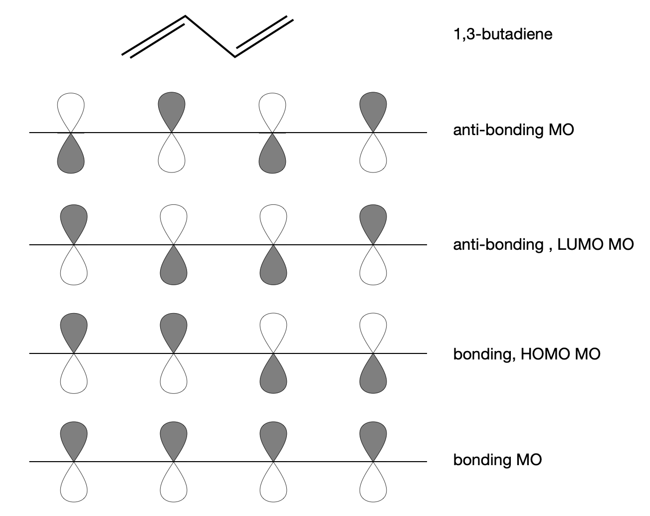
Figure 25. The bonding and anti-bonding molecular p\(\pi\) orbitals in butadiene are shown in order of increasing energy. The shading represents the relative phase component of the orbital often represented by + and -.

---

In butadiene there are only two classes of atoms, those at the end and those in the middle; therefore, by symmetry, only two constants \(a\) and \(b\) are needed, the vectors must have the form

\[\displaystyle \vec v=a\vec \pi_1 \pm +b\vec \pi_2 \pm +b\vec \pi_3 \pm +a\vec \pi_4 \]

and the \(\pm\) signs ensure orthogonality. The set of the base vectors is

\[\begin{split}\displaystyle \begin{bmatrix}\vec v_1& \vec v_2 & \vec v_3 & \vec v_4\end{bmatrix}=\begin{bmatrix}a\\b\\b\\a\end{bmatrix}\; \begin{bmatrix}b\\a\\-a\\-b\end{bmatrix}\; \begin{bmatrix}b\\-a\\-a\\b\end{bmatrix}\;\begin{bmatrix}a\\-b\\b\\-a\end{bmatrix} \end{split}\]

where each member of the basis set is itself a (column) vector and is an eigenvector from a Huckel calculation. The plus and minus pattern of the vector components is the same as the phase of the \(\pi\)-orbitals. In our previous calculations \(i, j, k\) base vectors were used, but when there are four or more base vectors, each with four or more terms, a matrix representation has to be used. We could, if so inclined, define a set of four orthogonal unit vectors, say, \(i, j, k, m\) and define their properties as for the three-dimensional vectors \(i, j, k\), and use these instead of the matrices but this would be very cumbersome.

As a check that the elements of our butadiene basis set are normalized, the dot product \(\vec v_1\cdot \vec v_1\) is

\[\begin{split}\displaystyle \vec v_1\cdot \vec v_1=\begin{bmatrix}a&b&b&a\end{bmatrix}\begin{bmatrix}a\\b\\b\\a\end{bmatrix}=2(a^2+b^2)\end{split}\]

The Huckel MO calculation (see in Chapter 7) produces values of \(a = 0.3717\) and \(b = 0.6015\) and as \(2(a^2 + b^2) = 1\) each vector is normalized. To check for orthogonality, calculate the dot product between any two vectors;

\[\begin{split}\displaystyle \vec v_3\cdot \vec v_1=\begin{bmatrix}b&-a&-a&b\end{bmatrix}\begin{bmatrix}a\\b\\b\\a\end{bmatrix}=0\end{split}\]

We have seen how linear combinations of molecular orbitals are used to represent p\(_x\) and p\(_y\) atomic orbitals, and the same is true in molecules. Linear combination or hybrid orbitals can always be formed because they are valid solutions of linear differential equations such as the Schroedinger equation. The combination \(\vec v_1 + \vec v_3\) produces

\[\begin{split}\displaystyle \vec v_{1+3}=\begin{bmatrix}a+b\\b-a\\b-a\\a+b\\ \end{bmatrix}\end{split}\]

with a dot product with itself of \(4(a^2 + b^2) = 2\), so this vector is normalized by dividing with \(1/\sqrt{2}\). The same result can be found by calculating with the base vectors \((\vec v_1 + \vec v_3)\cdot(\vec v_1 + \vec v_3) = 2\). The dot product with \(\vec v_2\) is

\[\begin{split}\displaystyle \vec v_2\cdot \vec v_{1+3} = \begin{bmatrix}b&a&-a&-b\end{bmatrix} \begin{bmatrix}a+b\\b-a\\b-a\\a+b\end{bmatrix}=0\end{split}\]

showing that this orbital is also orthogonal to the others that are not part of the linear combination. When orbitals are degenerate, forming linear combinations can be a more convenient way of viewing the orbitals. This is true in benzene where some of the familiar shapes of the Huckel MO’s are linear combinations; see matrices Q7 and Q50. To make a more accurate calculation of other orbitals besides the p\(\pi\), perhaps higher s or d orbitals must be added and then the basis set will have to expand. In molecular orbital calculations, a choice of predetermined basis sets of different complexity such as 631G can be used. Very often these basis sets consist of Gaussian functions (\(ae^{-bx^ 2}\)) parameterized with constants \(a\) and \(b\) to fit to Slater type atomic orbitals. Gaussian functions are used as they can be integrated easily. Huge basis sets containing millions of terms are necessary to represent molecular orbitals accurately and computer calculations of this type are very time consuming and among the most challenging of all calculations requiring super-computers.